About

A postdoc in theoretical particle physics, using LLMs to accelerate research

Author

Moises Zeleny

Physics background

Postdoc researcher at IF-UNAM, working in theoretical / particle physics with a focus on Beyond–the–Standard–Model (BSM) phenomenology, particularly in the context of extended scalar and gauge sectors. My research interests include neutrino masses, dark matter, and collider/flavour signatures. I am proficient in using tools such as SARAH, SPheno, FeynRules, MadGraph, micrOMEGAs, as well as programming in Python.

The Standard Model Lagrangian

The theory this log ultimately builds on, written by sector:

\[ \mathcal{L}_{\text{SM}} = \mathcal{L}_{\text{gauge}} + \mathcal{L}_{\text{fermion}} + \mathcal{L}_{\text{Higgs}} + \mathcal{L}_{\text{Yukawa}} \]

\[ \begin{aligned} \mathcal{L}_{\text{gauge}} &= -\tfrac{1}{4}\,G^{a}_{\mu\nu}G^{a\,\mu\nu} -\tfrac{1}{4}\,W^{i}_{\mu\nu}W^{i\,\mu\nu} -\tfrac{1}{4}\,B_{\mu\nu}B^{\mu\nu}, \\[4pt] \mathcal{L}_{\text{fermion}} &= i\,\bar{\psi}\,\gamma^{\mu} D_{\mu}\,\psi, \\[4pt] \mathcal{L}_{\text{Higgs}} &= (D_{\mu}\phi)^{\dagger}(D^{\mu}\phi) - V(\phi), \qquad V(\phi) = \mu^{2}\,\phi^{\dagger}\phi + \lambda\,(\phi^{\dagger}\phi)^{2}, \\[4pt] \mathcal{L}_{\text{Yukawa}} &= -\bigl(\bar{\psi}_{L}\,Y\,\psi_{R}\,\phi + \text{h.c.}\bigr). \end{aligned} \]

: where \(G\), \(W\), \(B\) are the \(SU(3)_C \times SU(2)_L \times U(1)_Y\) field strengths, \(D_\mu\) the gauge-covariant derivative, \(\phi\) the Higgs doublet, and \(Y\) the Yukawa matrices.

Beyond the Standard Model (BSM) physics is often explored by extending this Lagrangian with additional fields, symmetries, or interactions. My work focuses on analyzing these extensions and their phenomenological implications.

What a discovery looks like

The plot that made the Standard Model feel complete — and, for me, marks where Beyond-the-Standard-Model work begins. Below is an illustrative reconstruction of the H → γγ diphoton invariant-mass spectrum: a smoothly falling background with a narrow resonance near 125 GeV. The data here is synthetic (fixed random seed), not real experimental data — it’s a sketch of what the discovery looked like.

Show the code
import numpy as np
import matplotlib.pyplot as plt
from matplotlib import gridspec

# --- Academic styling to match the site ---------------------------------------
paper, ink, accent, grey = "#fcfcfa", "#22262b", "#3a5a7a", "#8a8f96"
plt.rcParams.update({
    "font.family": "serif",
    "font.size": 11,
    "axes.edgecolor": ink,
    "axes.linewidth": 0.8,
    "figure.facecolor": paper,
    "axes.facecolor": paper,
    "savefig.facecolor": paper,
})

# --- Illustrative H -> gamma gamma model --------------------------------------
# Falling background + a narrow resonance at m_H = 125 GeV. Numbers are
# representative, chosen for a clear bump; NOT fitted to real data.
binw = 2.0
edges = np.arange(100.0, 160.0 + binw, binw)      # 2 GeV bins over [100, 160] GeV
centers = 0.5 * (edges[:-1] + edges[1:])
rng = np.random.default_rng(125)

def background(m):
    return 2600.0 * np.exp(-0.045 * (m - 100.0))

def signal(m, mH=125.0, sigma=1.7, nsig=1100.0):
    gauss = np.exp(-0.5 * ((m - mH) / sigma) ** 2) / (sigma * np.sqrt(2 * np.pi))
    return nsig * gauss * binw                     # -> expected events per 2 GeV bin

bkg = background(centers)
expect = bkg + signal(centers)
data = rng.poisson(expect).astype(float)           # pseudo-data
err = np.sqrt(data)

mfine = np.linspace(100.0, 160.0, 400)
bkg_fine, sig_fine = background(mfine), signal(mfine)

# --- Two-panel figure ---------------------------------------------------------
fig = plt.figure(figsize=(6.4, 5.2))
gs = gridspec.GridSpec(2, 1, height_ratios=[3, 1], hspace=0.08)
ax, axr = fig.add_subplot(gs[0]), None
axr = fig.add_subplot(gs[1], sharex=ax)

ax.errorbar(centers, data, yerr=err, fmt="o", ms=4, color=ink, ecolor=grey,
            elinewidth=0.9, capsize=0, label="Data (synthetic)", zorder=3)
ax.plot(mfine, bkg_fine, "--", color=grey, lw=1.6, label="Background fit", zorder=2)
ax.plot(mfine, bkg_fine + sig_fine, "-", color=accent, lw=2.0,
        label="Signal + background fit", zorder=2)
ax.axvline(125, color=accent, lw=0.8, ls=":", alpha=0.6, zorder=1)
ax.set_ylabel("Events / 2 GeV")
ax.set_ylim(bottom=0)
ax.legend(frameon=False, fontsize=9, loc="upper right")
ax.tick_params(labelbottom=False)
ax.set_title(r"$H \rightarrow \gamma\gamma$  (illustrative, synthetic data)",
             fontsize=12, pad=8)

axr.errorbar(centers, data - bkg, yerr=err, fmt="o", ms=4, color=ink, ecolor=grey,
             elinewidth=0.9, capsize=0, zorder=3)
axr.plot(mfine, sig_fine, "-", color=accent, lw=2.0, zorder=2)
axr.axhline(0, color=grey, lw=0.8, zorder=1)
axr.set_ylabel(r"Data $-$ Bkg")
axr.set_xlabel(r"$m_{\gamma\gamma}$  [GeV]")

for a in (ax, axr):
    a.spines[["top", "right"]].set_visible(False)
    a.grid(axis="y", color=grey, alpha=0.15, lw=0.6)
    a.set_xlim(100, 160)

plt.show()
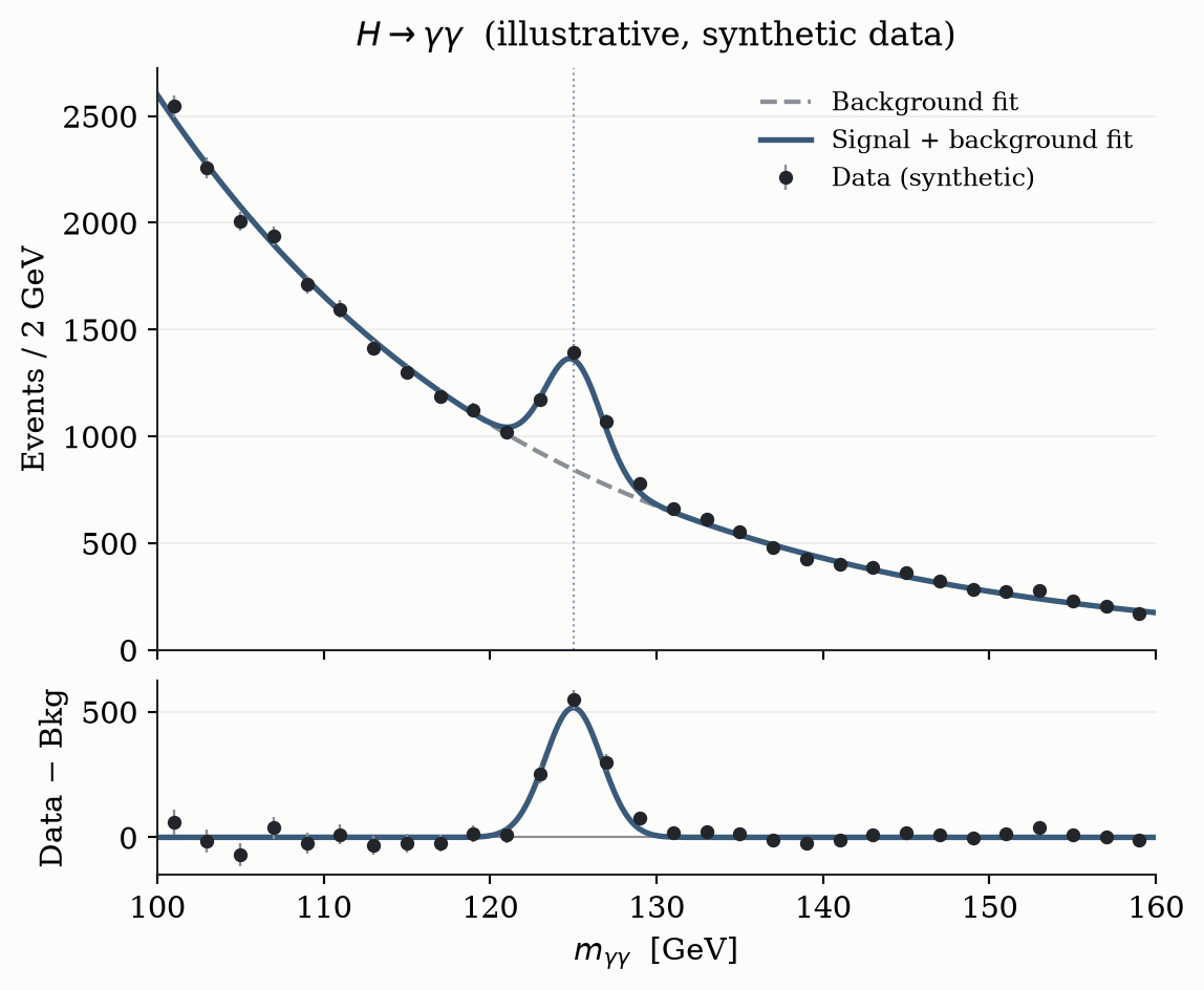
Figure 1: Illustrative H → γγ invariant-mass spectrum (synthetic data, fixed seed — not real experimental data). Top: pseudo-data with background-only (dashed) and signal+background (solid) fits. Bottom: background-subtracted excess with the fitted signal Gaussian at 125 GeV.

Why this log exists

I use large language models as part of my research workflow, and I wanted an honest, reproducible record of where they genuinely help and where they don’t — derivations, code, literature triage, model building — without the marketing gloss. See the first post for the longer statement of intent.

About the posts

Each entry documents a single real task: the tool and model used, the workflow, what worked, what failed, the time saved, and — wherever possible — a link to the code or notebook so you can reproduce it. Posts are written in English or Spanish.

Contact