Beyond the direct answer: an LLM + CAS workflow for theoretical physics

English
workflow
llms
cas
sympy
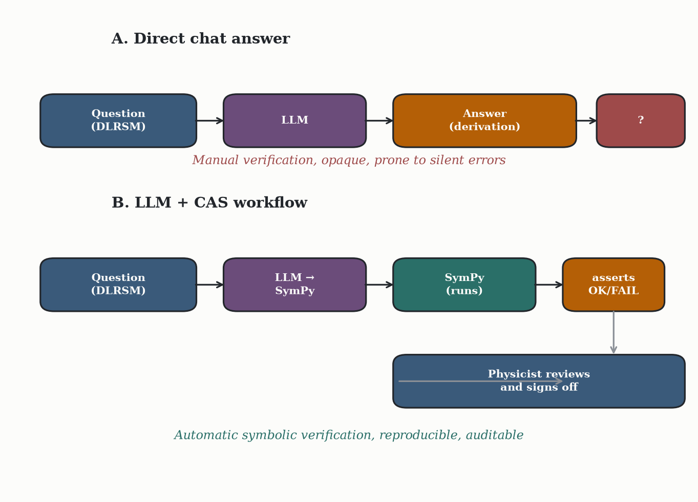
Comparing a direct chat answer with an LLM + SymPy workflow for the scalar-potential minimization of the DLRSM.
Author

Moises Zeleny

Published

August 2, 2026

Versión en español disponible. Este artículo también está disponible en español.

Abstract

This post tests a concrete workflow for doing theoretical-physics algebra with a large language model (LLM) without trusting its output blindly: ask the LLM to write SymPy code, then let the computer algebra system check every identity. The test case is the scalar-potential minimization of the Doublet Left-Right Symmetric Model (DLRSM). I compare the direct answer from a chat prompt (Gemini 3.1 Pro, 2026-08-02) against the LLM+CAS pipeline, and show that the latter produces a reproducible, assertion-checked derivation whose physical masses match the published results.

Motivation

In the previous post of this log why-this-log-exists I warned that large language models (LLMs) are particularly dangerous when they produce a derivation that looks correct but is wrong by a factor of \(1/(4\pi)^2\), a sign, or a convention. The only defense I know is to do the calculation yourself and treat the model’s output as a hypothesis to be tested.

The problem is that, for many theoretical-physics problems, “verifying” by hand takes as much time as doing the original calculation. The traditional workflow is, in practice, oracular: you ask the model, it gives an answer, and then you either trust it or redo it. What I propose here is a constructive workflow:

  1. Do not ask the LLM for the final answer.
  2. Ask it to write the code (SymPy) that produces the answer.
  3. Run that code in a computer algebra system (CAS).
  4. Explicitly verify the identities the CAS can check: tadpole conditions, Goldstone eigenvalues, physical masses, agreement with published equations.

The CAS does not remove the physicist’s responsibility; it shifts it: from “do the calculation by hand” to “write a verification harness that the CAS evaluates symbolically”. This is the same spirit as recent work such as Hell and Thiele (2026), where LLMs are used as translators of intent into symbolic code, not as oracles.

The test case: scalar-potential minimization in the DLRSM

The model is the Doublet Left-Right Symmetric Model (DLRSM), described in Zeleny-Mora et al. (2026). The scalar sector contains a bidoublet \(\Phi\) and two doublets \(\chi_L, \chi_R\) with VEVs

\[ \langle\Phi\rangle = \mathrm{diag}(k_1, k_2), \qquad \langle\chi_L\rangle = \begin{pmatrix}0\\ v_L\end{pmatrix}, \qquad \langle\chi_R\rangle = \begin{pmatrix}0\\ v_R\end{pmatrix}. \]

The scalar potential, taken from Senjanović (1979) and used in Zeleny-Mora et al. (2026), is \(V = V_\Phi + V_\chi + V_{\Phi\chi}\) with

\[ \begin{aligned} V_\Phi =& -\mu_1^2 \mathrm{Tr}\Phi^\dagger\Phi + \lambda_1 \left(\mathrm{Tr}\Phi^\dagger\Phi\right)^2 + \lambda_2 \mathrm{Tr}\Phi^\dagger\Phi\Phi^\dagger\Phi \\& + \frac{\lambda_3}{2}\left(\mathrm{Tr}\Phi^\dagger\tilde\Phi + \mathrm{Tr}\tilde\Phi^\dagger\Phi\right)^2 + \frac{\lambda_4}{2}\left(\mathrm{Tr}\Phi^\dagger\tilde\Phi - \mathrm{Tr}\tilde\Phi^\dagger\Phi\right)^2 \\& + \lambda_5 \mathrm{Tr}\Phi^\dagger\Phi\tilde\Phi^\dagger\tilde\Phi + \frac{\lambda_6}{2}\left[\mathrm{Tr}\Phi^\dagger\tilde\Phi\Phi^\dagger\tilde\Phi + \mathrm{h.c.}\right], \end{aligned} \]

\[ V_\chi = -\mu_2^2\left(\chi_L^\dagger\chi_L + \chi_R^\dagger\chi_R\right) + \rho_1\left[\left(\chi_L^\dagger\chi_L\right)^2 + \left(\chi_R^\dagger\chi_R\right)^2\right] + \rho_2\,\chi_L^\dagger\chi_L\,\chi_R^\dagger\chi_R, \]

\[ \begin{aligned} V_{\Phi\chi} =& \;\alpha_1\,\mathrm{Tr}\Phi^\dagger\Phi\left(\chi_L^\dagger\chi_L + \chi_R^\dagger\chi_R\right) \\& + \alpha_2\left(\chi_L^\dagger\Phi\Phi^\dagger\chi_L + \chi_R^\dagger\Phi^\dagger\Phi\chi_R\right) \\& + \alpha_3\left(\chi_L^\dagger\tilde\Phi\tilde\Phi^\dagger\chi_L + \chi_R^\dagger\tilde\Phi^\dagger\tilde\Phi\chi_R\right). \end{aligned} \]

Definitions: from the potential to the masses

The computation of the scalar masses from \(V\) follows a standard four-step chain, which the CAS will verify at every link.

  1. Expansion around the vacuum. Each scalar is written as its VEV plus a fluctuation, for example \[ \phi_i^0(x) = \frac{1}{\sqrt{2}}\big(v_i + \eta_i(x) + i\,\xi_i(x)\big). \] The potential is then expanded to quadratic order in the fluctuations; the bilinear part defines the mass spectrum.

  2. Tadpole conditions (stationarity). The VEVs \(\{k_1, k_2, v_L, v_R\}\) are fixed by requiring the vacuum to be an extremum: \[ \frac{\partial V}{\partial v_i}\bigg|_{\mathrm{VEV}} = 0, \qquad v_i \in \{k_1, k_2, v_L, v_R\}. \] When these are satisfied, the linear terms in the expansion of \(V\) — the tadpoles — vanish identically.

  3. Mass matrix (Hessian of the potential). The squared-mass matrix is the Hessian of \(V\) evaluated at the vacuum. For the neutral scalars (real components \(\varphi_i = \{\eta_i, \xi_i\}\)), \[ \big(M^2\big)_{ij} = \frac{\partial^2 V}{\partial \varphi_i\,\partial \varphi_j}\bigg|_{\mathrm{VEV}}. \] For the charged sector the fields are complex, and the Wirtinger convention is used: \[ \big(M_+^2\big)_{ij} = \frac{\partial^2 V}{\partial c_i^{+}\,\partial c_j^{-}}\bigg|_{\mathrm{VEV}}, \qquad c^{\pm} = (\phi_2^{\pm}, \chi_L^{\pm}, \phi_1^{\pm}, \chi_R^{\pm}), \] where \(c_i^+\) and \(c_j^-\) are treated as independent variables. The tadpole conditions are substituted into \(M^2\) to eliminate the bare mass parameters \(\mu_{1,2}^2\).

  4. Goldstone bosons and physical masses. By Goldstone’s theorem, each spontaneously broken gauge generator produces a massless mode that becomes the longitudinal polarization of a massive gauge boson. In the charged sector of the DLRSM, the breaking of \(SU(2)_L \times SU(2)_R\) down to \(U(1)_{\mathrm{em}}\) leaves two charged Goldstones \(G_L^\pm, G_R^\pm\) — eaten by \(W_L^\pm\) and \(W_R^\pm\) — so \(M_+^2\) must have exactly two zero eigenvalues. The remaining non-zero eigenvalues are the squared masses of the physical charged Higgs bosons \(H_{L,R}^\pm\).

The concrete problem I will pose to the LLM is: derive the four tadpole conditions, the charged-scalar mass matrix in the limit \(v_L = k_2 = 0\), and the physical charged Higgs masses.

Arm A: direct answer from a chat

I used the model Gemini 3.1 Pro on 2026-08-02 with the following prompt (also in the post’s Appendix):

Consider the Doublet Left-Right Symmetric Model with a bidoublet \(\Phi = [\phi_1, i\sigma_2\phi_2^*]\) with \(\langle\Phi\rangle = \mathrm{diag}(k_1, k_2)\) and doublets \(\chi_{L,R}\) with \(\langle\chi_{L,R}^0\rangle = v_{L,R}\). The scalar potential is \(V = V_\Phi + V_\chi + V_{\Phi\chi}\) where [full potential]. Derive: (a) the four tadpole conditions; (b) the charged scalar mass matrix in the basis \((\phi_2^+, \chi_L^+, \phi_1^+, \chi_R^+)\) in the limit \(v_L = k_2 = 0\); (c) the physical charged Higgs masses.

The answer is impressive at first sight: correct structure, plausible parameter combinations, and final physical masses that match the literature. I transcribe the main results here (abbreviated; the full text is in the folded block):

To derive the properties of the scalar sector in this Left-Right Symmetric Model (LRSM), we evaluate the scalar potential \(V = V_\Phi + V_\chi + V_{\Phi\chi}\) using the standard field expansions around the vacuum expectation values (VEVs).

The bidoublet \(\Phi\) and the left/right doublets \(\chi_{L,R}\) are given by: \[ \Phi = \begin{pmatrix} \phi_1^0 & \phi_2^+ \\ \phi_1^- & \phi_2^0 \end{pmatrix}, \quad \chi_L = \begin{pmatrix} \chi_L^+ \\ \chi_L^0 \end{pmatrix}, \quad \chi_R = \begin{pmatrix} \chi_R^+ \\ \chi_R^0 \end{pmatrix} \] where \(\tilde{\Phi} = \sigma_2 \Phi^* \sigma_2 = \begin{pmatrix} \phi_2^{0*} & -\phi_1^+ \\ -\phi_2^- & \phi_1^{0*} \end{pmatrix}\).

(a) The Four Tadpole Conditions. Minimizing the potential with respect to the non-zero VEVs yields \[ \mu_1^2 = 2\lambda_1(k_1^2+k_2^2) + 2\lambda_2k_1^2 + (8\lambda_3+2\lambda_5+2\lambda_6)k_2^2 + (\alpha_1+\alpha_3)(v_L^2+v_R^2), \] and the corresponding equations for \(k_2, v_L, v_R\).

(b) Charged Scalar Mass Matrix (\(v_L = k_2 = 0\)). In the basis \((\phi_2^+, \chi_L^+, \phi_1^+, \chi_R^+)\), \[ M^2 = \begin{pmatrix} (\alpha_2-\alpha_3) v_R^2 & 0 & 0 & (\alpha_2-\alpha_3) k_1 v_R \\ 0 & (\rho_2-2\rho_1) v_R^2 + (\alpha_2-\alpha_3) k_1^2 & 0 & 0 \\ 0 & 0 & 0 & 0 \\ (\alpha_2-\alpha_3) k_1 v_R & 0 & 0 & (\alpha_2-\alpha_3) k_1^2 \end{pmatrix}. \]

(c) Physical Charged Higgs Masses. \[ M_{H_1^\pm}^2 = (\rho_2-2\rho_1)v_R^2 + (\alpha_2-\alpha_3)k_1^2, \qquad M_{H_2^\pm}^2 = (\alpha_2-\alpha_3)(v_R^2+k_1^2). \]

Gemini identifies \(\phi_1^+\) as the Goldstone boson \(G_L^\pm\) and the \((\phi_2^+, \chi_R^+)\) block as the \(G_R^\pm/H_2^\pm\) mixing.

The answer is superficially correct: the final masses agree with the published equations in Zeleny-Mora et al. (2026, Eq. (13)). The problem is that, as a reader, I cannot tell whether the matrix structure is correct without redoing the algebra. The model’s errors are of the hardest kind to detect: not grammatical mistakes or obvious inconsistencies, but silent errors hidden inside a structure that looks right.

Arm B: LLM + CAS with SymPy

The same problem is posed to the LLM in a different mode: “do not give me the answer; write me the SymPy code that computes it”. The code is shown in the following cell (folded) and is executed as part of the post. The table maps each theoretical step of the Definitions section to the SymPy idiom that implements it and the check the CAS performs:

Theory step In the code What the CAS verifies
0. Encode the potential \(V\) fields as Matrix objects; trace(...) builds \(V_\Phi+V_\chi+V_{\Phi\chi}\)
1. Expansion around the vacuum V.subs(VEV_all) sets \(\langle\Phi\rangle=\mathrm{diag}(k_1,k_2)\), \(\langle\chi^0_{L,R}\rangle=v_{L,R}\)
2. Tadpole conditions \(\partial V/\partial v_i=0\) sp.diff(V0, k1), … over the four VEVs matches Eq. (9) of Zeleny-Mora et al. (2026)
3. Mass matrix (Wirtinger Hessian) sp.diff(V, c_plus[i], c_minus[j]); \(\mu_{1,2}^2\) eliminated via the tadpoles structure of \(M_+^2\) in the \(v_L=k_2=0\) limit
4. Goldstones and physical masses M_charged.charpoly(lam) \(\lambda^2(\lambda-m^2_{H_L^\pm})(\lambda-m^2_{H_R^\pm})\): two zero modes + Eq. (13)

Two design choices mirror the theory directly. First, each complex field and its conjugate are declared as separate real symbolsphi1m and phi1mc, chiL and chiLc, … This is precisely the Wirtinger prescription of step 3: \(c_i^+\) and \(c_j^-\) are independent variables, so the Hessian sp.diff(V, c_plus[i], c_minus[j]) differentiates with respect to a field and its conjugate as if unrelated. Second, the step-4 Goldstone check does not ask SymPy for eigenvalues — symbolic eigenvalues of a \(4\times4\) matrix can be unruly radicals — but compares the characteristic polynomial against \(\lambda^2(\lambda-m^2_{H_L^\pm})(\lambda-m^2_{H_R^\pm})\), a polynomial identity that simplify can decide exactly, turning “are there exactly two zero modes?” into algebra. Every assert is such a check; if one fails, the cell throws an exception instead of producing a silently wrong answer.

Show the SymPy code
import sympy as sp
from sympy import symbols, Matrix, simplify, factor, trace, expand
from IPython.display import display, Math

# --- Symbols ----------------------------------------------------------------
# We use real variables for each complex field and its conjugate.
phi10, phi10c = symbols('phi10 phi10c', real=True)   # phi_1^0, phi_1^{0*}
phi20, phi20c = symbols('phi20 phi20c', real=True)   # phi_2^0, phi_2^{0*}
phi1m, phi1mc = symbols('phi1m phi1mc', real=True)   # phi_1^-, phi_1^+
phi2m, phi2mc = symbols('phi2m phi2mc', real=True)   # phi_2^-, phi_2^+
chiL, chiLc     = symbols('chiL chiLc', real=True)   # chi_L^+, chi_L^-
chiR, chiRc     = symbols('chiR chiRc', real=True)   # chi_R^+, chi_R^-
chiLn, chiLnc  = symbols('chiLn chiLnc', real=True) # chi_L^0, chi_L^{0*}
chiRn, chiRnc  = symbols('chiRn chiRnc', real=True) # chi_R^0, chi_R^{0*}

mu1sq, mu2sq = symbols('{{\\mu_{1}^2}} {{\\mu_{2}^2}}', positive=True)
lam1, lam2, lam3, lam4, lam5, lam6 = symbols('lambda_1 lambda_2 lambda_3 lambda_4 lambda_5 lambda_6', real=True)
rho1, rho2 = symbols('rho1 rho2', real=True)
alpha1, alpha2, alpha3 = symbols('alpha1 alpha2 alpha3', real=True)

k1, k2, vL, vR = symbols('k_1 k_2 v_L v_R', positive=True)

# --- Bidoublet and doublet matrices -----------------------------------------
# Phi = [phi_1, i*sigma2*phi_2^*]
Phi = Matrix([
    [phi10, phi2mc],
    [phi1m, -phi20c]
])
Phi_dag = Matrix([
    [phi10c, phi1mc],
    [phi2m,  -phi20]
])

I = sp.I
sigma2 = Matrix([[0, -I], [I, 0]])
Phi_star = Matrix([[phi10c, phi2m], [phi1mc, -phi20]])
tilde_Phi = sigma2 * Phi_star * sigma2
tilde_Phi_dag = sigma2 * Phi.T * sigma2

chi_L = Matrix([[chiL], [chiLn]])
chi_L_dag = Matrix([[chiLc, chiLnc]])
chi_R = Matrix([[chiR], [chiRn]])
chi_R_dag = Matrix([[chiRc, chiRnc]])

# --- Scalar potential ---------------------------------------------------------
V_Phi = (
    -mu1sq * trace(Phi_dag * Phi)
    + lam1 * trace(Phi_dag * Phi)**2
    + lam2 * trace(Phi_dag * Phi * Phi_dag * Phi)
    + sp.Rational(1,2) * lam3 * (trace(Phi_dag * tilde_Phi) + trace(tilde_Phi_dag * Phi))**2
    + sp.Rational(1,2) * lam4 * (trace(Phi_dag * tilde_Phi) - trace(tilde_Phi_dag * Phi))**2
    + lam5 * trace(Phi_dag * Phi * tilde_Phi_dag * tilde_Phi)
    + sp.Rational(1,2) * lam6 * (trace(Phi_dag * tilde_Phi * Phi_dag * tilde_Phi)
                               + trace(tilde_Phi_dag * Phi * tilde_Phi_dag * Phi))
)

V_chi = (
    -mu2sq * (chi_L_dag.dot(chi_L) + chi_R_dag.dot(chi_R))
    + rho1 * (chi_L_dag.dot(chi_L)**2 + chi_R_dag.dot(chi_R)**2)
    + rho2 * (chi_L_dag.dot(chi_L)) * (chi_R_dag.dot(chi_R))
)

V_Phi_chi = (
    alpha1 * trace(Phi_dag * Phi) * (chi_L_dag.dot(chi_L) + chi_R_dag.dot(chi_R))
    + alpha2 * (chi_L_dag * Phi * Phi_dag * chi_L + chi_R_dag * Phi_dag * Phi * chi_R)[0]
    + alpha3 * (chi_L_dag * tilde_Phi * tilde_Phi_dag * chi_L
                + chi_R_dag * tilde_Phi_dag * tilde_Phi * chi_R)[0]
)

V = expand(V_Phi + V_chi + V_Phi_chi)

# --- Tadpole: verification against Eq. (9) of the paper ---------------------
VEV_all = {
    phi10: k1, phi10c: k1, phi20: k2, phi20c: k2,
    phi1m: 0, phi1mc: 0, phi2m: 0, phi2mc: 0,
    chiL: 0, chiLc: 0, chiR: 0, chiRc: 0,
    chiLn: vL, chiLnc: vL, chiRn: vR, chiRnc: vR
}
V0 = V.subs(VEV_all)

lam12 = lam1 + lam2
lam1356 = lam1 + 4*lam3 + lam5 + lam6
alpha12 = alpha1 + alpha2
alpha13 = alpha1 + alpha3

paper_tadpoles = {
    'k1': 2*k1*(-mu1sq + 2*k1**2*lam12 + 2*k2**2*lam1356 + (vL**2 + vR**2)*alpha13),
    'k2': 2*k2*(-mu1sq + 2*k1**2*lam1356 + 2*k2**2*lam12 + (vL**2 + vR**2)*alpha12),
    'vL': 2*vL*(-mu2sq + 2*rho1*vL**2 + rho2*vR**2 + k1**2*alpha13 + k2**2*alpha12),
    'vR': 2*vR*(-mu2sq + 2*rho1*vR**2 + rho2*vL**2 + k1**2*alpha13 + k2**2*alpha12),
}

tadpoles = {
    'k1': sp.diff(V0, k1),
    'k2': sp.diff(V0, k2),
    'vL': sp.diff(V0, vL),
    'vR': sp.diff(V0, vR),
}

for key in tadpoles:
    diff = simplify(tadpoles[key] - paper_tadpoles[key])
    assert diff == 0, f"Tadpole {key} does not match the literature: {diff}"

print("✓ Tadpole conditions: match Eq. (9) of Zeleny-Mora et al. (2026)\n")
for label, key in [(r"k_1", "k1"), (r"k_2", "k2"), (r"v_L", "vL"), (r"v_R", "vR")]:
    display(Math(rf"\frac{{\partial V}}{{\partial {label}}} = " + sp.latex(factor(tadpoles[key]))))

# --- Solve for mu1^2 and mu2^2 in the vL = k2 = 0 limit ----------------------
mu1sq_sol = sp.solve(sp.Eq(tadpoles['k1'].subs({k2:0, vL:0}), 0), mu1sq)[0]
mu2sq_sol = sp.solve(sp.Eq(tadpoles['vR'].subs({k2:0, vL:0}), 0), mu2sq)[0]

assert simplify(mu1sq_sol - (2*k1**2*lam12 + vR**2*alpha13)) == 0
assert simplify(mu2sq_sol - (2*rho1*vR**2 + k1**2*alpha13)) == 0
print("✓ Mass parameters in the $v_L = k_2 = 0$ limit:\n")
display(Math(r"\mu_1^2 = " + sp.latex(mu1sq_sol)))
display(Math(r"\mu_2^2 = " + sp.latex(mu2sq_sol)))

# --- Charged scalar mass matrix ---------------------------------------------
# Basis c+ = (phi2+, chiL+, phi1+, chiR+)
# Mapping: phi2+ = phi2mc, chiL+ = chiL, phi1+ = phi1mc, chiR+ = chiR
c_plus = [phi2mc, chiL, phi1mc, chiR]
c_minus = [phi2m, chiLc, phi1m, chiRc]

M_charged = Matrix([[sp.diff(V, c_plus[i], c_minus[j]) for j in range(4)] for i in range(4)])

VEV_charged = {
    phi10: k1, phi10c: k1, phi20: 0, phi20c: 0,
    phi1m: 0, phi1mc: 0, phi2m: 0, phi2mc: 0,
    chiL: 0, chiLc: 0, chiR: 0, chiRc: 0,
    chiLn: 0, chiLnc: 0, chiRn: vR, chiRnc: vR
}
M_charged = M_charged.subs(VEV_charged).subs({mu1sq: mu1sq_sol, mu2sq: mu2sq_sol})
M_charged = simplify(M_charged)

print("\nCharged scalar mass matrix (basis $c^+ = (\\phi_2^+, \\chi_L^+, \\phi_1^+, \\chi_R^+)$):")
display(Math(r"M_+^2 = " + sp.latex(M_charged)))

# --- Physical verification: masses and Goldstones ---------------------------
alpha23 = alpha2 - alpha3
rho21 = rho2 - 2*rho1

# Physical masses expected from Eq. (13)
mH1_sq = k1**2*alpha23 + vR**2*rho21
mH2_sq = alpha23*(k1**2 + vR**2)

# Physical verification: two Goldstones and two correct physical masses.
# The characteristic polynomial must be lambda^2 * (lambda - mH1^2) * (lambda - mH2^2).
# This is more robust than counting zero eigenvalues symbolically,
# because SymPy may return a complicated expression that simplifies to zero.
lam = symbols('lam')
char_poly = M_charged.charpoly(lam).as_expr()
expected_poly = lam**2 * (lam - mH1_sq) * (lam - mH2_sq)
assert simplify(expand(char_poly - expected_poly)) == 0
print("\n✓ Characteristic polynomial: $\\lambda^2 (\\lambda - m^2_{H_L})(\\lambda - m^2_{H_R})$")
print("  → two zero eigenvalues (Goldstones) and two physical masses\n")
print("Physical charged masses:")
display(Math(r"m^2_{H_L^\pm} = " + sp.latex(mH1_sq)))
display(Math(r"m^2_{H_R^\pm} = " + sp.latex(mH2_sq)))
✓ Tadpole conditions: match Eq. (9) of Zeleny-Mora et al. (2026)

\(\displaystyle \frac{\partial V}{\partial k_1} = 2 k_{1} \left(\alpha_{1} v_{L}^{2} + \alpha_{1} v_{R}^{2} + \alpha_{3} v_{L}^{2} + \alpha_{3} v_{R}^{2} + 2 k_{1}^{2} \lambda_{1} + 2 k_{1}^{2} \lambda_{2} + 2 k_{2}^{2} \lambda_{1} + 8 k_{2}^{2} \lambda_{3} + 2 k_{2}^{2} \lambda_{5} + 2 k_{2}^{2} \lambda_{6} - {{\mu_{1}^2}}\right)\)

\(\displaystyle \frac{\partial V}{\partial k_2} = 2 k_{2} \left(\alpha_{1} v_{L}^{2} + \alpha_{1} v_{R}^{2} + \alpha_{2} v_{L}^{2} + \alpha_{2} v_{R}^{2} + 2 k_{1}^{2} \lambda_{1} + 8 k_{1}^{2} \lambda_{3} + 2 k_{1}^{2} \lambda_{5} + 2 k_{1}^{2} \lambda_{6} + 2 k_{2}^{2} \lambda_{1} + 2 k_{2}^{2} \lambda_{2} - {{\mu_{1}^2}}\right)\)

\(\displaystyle \frac{\partial V}{\partial v_L} = 2 v_{L} \left(\alpha_{1} k_{1}^{2} + \alpha_{1} k_{2}^{2} + \alpha_{2} k_{2}^{2} + \alpha_{3} k_{1}^{2} + 2 \rho_{1} v_{L}^{2} + \rho_{2} v_{R}^{2} - {{\mu_{2}^2}}\right)\)

\(\displaystyle \frac{\partial V}{\partial v_R} = 2 v_{R} \left(\alpha_{1} k_{1}^{2} + \alpha_{1} k_{2}^{2} + \alpha_{2} k_{2}^{2} + \alpha_{3} k_{1}^{2} + 2 \rho_{1} v_{R}^{2} + \rho_{2} v_{L}^{2} - {{\mu_{2}^2}}\right)\)

✓ Mass parameters in the $v_L = k_2 = 0$ limit:

\(\displaystyle \mu_1^2 = \alpha_{1} v_{R}^{2} + \alpha_{3} v_{R}^{2} + 2 k_{1}^{2} \lambda_{1} + 2 k_{1}^{2} \lambda_{2}\)

\(\displaystyle \mu_2^2 = \alpha_{1} k_{1}^{2} + \alpha_{3} k_{1}^{2} + 2 \rho_{1} v_{R}^{2}\)


Charged scalar mass matrix (basis $c^+ = (\phi_2^+, \chi_L^+, \phi_1^+, \chi_R^+)$):

\(\displaystyle M_+^2 = \left[\begin{matrix}v_{R}^{2} \left(\alpha_{2} - \alpha_{3}\right) & 0 & 0 & k_{1} v_{R} \left(\alpha_{2} - \alpha_{3}\right)\\0 & \alpha_{2} k_{1}^{2} - \alpha_{3} k_{1}^{2} - 2 \rho_{1} v_{R}^{2} + \rho_{2} v_{R}^{2} & 0 & 0\\0 & 0 & 0 & 0\\k_{1} v_{R} \left(\alpha_{2} - \alpha_{3}\right) & 0 & 0 & k_{1}^{2} \left(\alpha_{2} - \alpha_{3}\right)\end{matrix}\right]\)


✓ Characteristic polynomial: $\lambda^2 (\lambda - m^2_{H_L})(\lambda - m^2_{H_R})$
  → two zero eigenvalues (Goldstones) and two physical masses

Physical charged masses:

\(\displaystyle m^2_{H_L^\pm} = k_{1}^{2} \left(\alpha_{2} - \alpha_{3}\right) + v_{R}^{2} \left(- 2 \rho_{1} + \rho_{2}\right)\)

\(\displaystyle m^2_{H_R^\pm} = \left(\alpha_{2} - \alpha_{3}\right) \left(k_{1}^{2} + v_{R}^{2}\right)\)
Comparing the two arms

The difference is subtle but decisive. The chat model returns an answer that passes a quick review: the final masses are correct and the notation matches the paper. However, the answer has the properties that make an LLM dangerous in physics:

  • It is opaque. There is no reproducible path to it. To know if it is correct, the reader must redo all the algebra.
  • It is fragile in structure. Even when the final masses agree, the assignment of fields to physical states (Goldstone vs. Higgs) depends on the exact matrix structure. Without a CAS, a sign, a column swap, or a factor of 2 can go unnoticed.
  • It is not auditable. There is no “reproduce” button.

In contrast, the LLM+CAS workflow gives:

  • Full transparency. The code is the calculation; anyone can run it.
  • Automatic verification. Every assert is a check the CAS evaluates symbolically. If the LLM had written code with a wrong sign, the cell would have failed with an error message, not produced a plausible-looking answer.
  • Traceability. The relation between the potential, the tadpole conditions, the mass matrix, and the physical masses is explicit and readable.

Toward the theoretical physicist’s workflow in the LLM era

Show the figure code
import matplotlib.pyplot as plt
import matplotlib.patches as mpatches
from matplotlib.patches import FancyBboxPatch, FancyArrowPatch

paper, ink, accent, grey = "#fcfcfa", "#22262b", "#3a5a7a", "#8a8f96"
red, green = "#9e4a4a", "#2a6f68"

plt.rcParams.update({
    "font.family": "serif",
    "font.size": 10,
    "axes.edgecolor": ink,
    "axes.linewidth": 0.8,
    "figure.facecolor": paper,
    "axes.facecolor": paper,
    "savefig.facecolor": paper,
})

fig, ax = plt.subplots(figsize=(7.2, 5.2))
ax.set_xlim(0, 10)
ax.set_ylim(0, 10)
ax.axis("off")

def box(x, y, w, h, text, color=accent, text_color=paper):
    rect = FancyBboxPatch((x, y), w, h, boxstyle="round,pad=0.05,rounding_size=0.2",
                          facecolor=color, edgecolor=ink, linewidth=1.2)
    ax.add_patch(rect)
    ax.text(x + w/2, y + h/2, text, ha="center", va="center", color=text_color,
            fontsize=8, weight="bold", wrap=True)

def arrow(x1, y1, x2, y2, color=ink, style="->"):
    ax.annotate("", xy=(x2, y2), xytext=(x1, y1),
                arrowprops=dict(arrowstyle=style, color=color, lw=1.2))

# --- Arm A: direct chat answer ----------------------------------------------
ax.text(1.5, 9.3, "A. Direct chat answer", fontsize=11, weight="bold", color=ink)
box(0.5, 7.2, 2.2, 1.0, "Question\n(DLRSM)", accent)
box(3.2, 7.2, 2.0, 1.0, "LLM", "#6b4c7a")
box(5.7, 7.2, 2.6, 1.0, "Answer\n(derivation)", "#b45f06")
box(8.7, 7.2, 1.2, 1.0, "?", red)
arrow(2.7, 7.7, 3.2, 7.7)
arrow(5.2, 7.7, 5.7, 7.7)
arrow(8.3, 7.7, 8.7, 7.7)
ax.text(5.0, 6.8, "Manual verification, opaque, prone to silent errors",
        ha="center", fontsize=9, color=red, style="italic")

# --- Arm B: LLM + CAS -------------------------------------------------------
ax.text(1.5, 5.9, "B. LLM + CAS workflow", fontsize=11, weight="bold", color=ink)
box(0.5, 3.8, 2.2, 1.0, "Question\n(DLRSM)", accent)
box(3.2, 3.8, 2.0, 1.0, "LLM →\nSymPy", "#6b4c7a")
box(5.7, 3.8, 2.0, 1.0, "SymPy\n(runs)", green)
box(8.2, 3.8, 1.4, 1.0, "asserts\nOK/FAIL", "#b45f06")
box(5.7, 1.8, 4.2, 1.0, "Physicist reviews\nand signs off", accent)

arrow(2.7, 4.3, 3.2, 4.3)
arrow(5.2, 4.3, 5.7, 4.3)
arrow(7.7, 4.3, 8.2, 4.3)
# Feedback loop
arrow(8.9, 3.8, 8.9, 2.8, color=grey)
arrow(8.2, 2.3, 5.7, 2.3, color=grey, style="<-")
ax.text(5.0, 1.1, "Automatic symbolic verification, reproducible, auditable",
        ha="center", fontsize=9, color=green, style="italic")

plt.tight_layout()
Figure 1: Workflow comparison. Top: direct chat answer — the physicist must verify by hand, and errors are silent. Bottom: LLM generates SymPy code, the CAS runs symbolic asserts, and the physicist reviews and signs off.

The DLRSM case is a clean example of the broader pattern. The CAS does not replace the physicist; it defines a division of responsibilities:

Task LLM CAS Physicist
Translate the physics question into a script Yes No Supervise
Execute exact symbolic algebra No Yes Design the verification harness
Decide what to check and what it means physically No No Yes
Detect convention, sign, or factor errors Partially Yes Yes
Produce a reproducible derivation Only as code Yes Yes

This pattern scales in several directions. Today SymPy covers the polynomial algebra of the scalar sector; for one-loop calculations with Passarino–Veltman functions, the same workflow points to tools like FeynCalc, Package-X, or LoopTools, with the LLM acting as an orchestrator between them. This is where work such as Hell and Thiele (2026) explores the frontier: not an LLM that solves the problem, but an LLM that writes the code the CAS runs and the physicist verifies.

The deepest change is cultural. In the near future, a PhD student in theoretical physics will likely spend less time rewriting matrix products by hand and more time on:

  1. Formulating the model and the verification protocol.
  2. Asking an LLM to generate the CAS code.
  3. Running the code, checking the assert, and analyzing the limiting cases.
  4. Deciding whether the result makes physical sense.

The derivation does not disappear; it becomes code. And code, unlike a chat answer, can be run, audited, and fixed.

Honest limits

The workflow is not infallible. The CAS only checks what we ask it to check. If the LLM writes code that typechecks but encodes the wrong physics—for example, using the wrong invariant in the potential—the assert will pass and the physical result will be wrong. The CAS does not replace physical judgment; it formalizes it.

There are also practical limitations:

  • Context and length: for potentials with dozens of parameters, the prompt can become unwieldy.
  • SymPy performance: real loop integrals or very large matrices quickly exceed what SymPy can do in reasonable time.
  • Conventions: the LLM may mix up sign conventions for \(\tilde\Phi\), \(\tau\), or charges. The verification harness should include at least a gauge-invariance check or a known limit.

The point is not that LLM+CAS does everything. The point is that it converts the model’s uncertainty into a CAS exception, which is much easier to diagnose than a plausibly wrong answer.

This post contains a {python} cell executed locally with SymPy Meurer et al. (2017). The frozen results are stored in _freeze/posts/llm-cas-workflow/ and committed with the .qmd. The CI runner only has Quarto, no Python, so any change to the cell must be re-rendered locally. The full prompt to Gemini 3.1 Pro is in the Appendix; the transcribed response was used as-is on 2026-08-02. No numerical results from ongoing projects are included: the example uses only the published symbolic equations from Zeleny-Mora et al. (2026).

Appendix: full prompt to Gemini 3.1 Pro

The prompt was sent on 2026-08-02 to the Gemini 3.1 Pro model. The response text was abbreviated in the body of the post; the full prompt is reproduced here so anyone can repeat it:

Consider the Doublet Left-Right Symmetric Model (DLRSM) with a bidoublet \(\Phi = [\phi_1, i\sigma_2\phi_2^*]\) where \(\phi_i = (\phi_i^0, \phi_i^-)^T\), and \(\langle\Phi\rangle = \mathrm{diag}(k_1, k_2)\). The model also contains two doublets \(\chi_L = (\chi_L^+, \chi_L^0)^T\) and \(\chi_R = (\chi_R^+, \chi_R^0)^T\) with \(\langle\chi_L^0\rangle = v_L\) and \(\langle\chi_R^0\rangle = v_R\). The scalar potential is \(V = V_\Phi + V_\chi + V_{\Phi\chi}\) where \[ \begin{aligned} V_\Phi =& -\mu_1^2 \mathrm{Tr}\Phi^\dagger\Phi + \lambda_1 \left(\mathrm{Tr}\Phi^\dagger\Phi\right)^2 + \lambda_2 \mathrm{Tr}\Phi^\dagger\Phi\Phi^\dagger\Phi \\& + \frac{\lambda_3}{2}\left(\mathrm{Tr}\Phi^\dagger\tilde\Phi + \mathrm{Tr}\tilde\Phi^\dagger\Phi\right)^2 + \frac{\lambda_4}{2}\left(\mathrm{Tr}\Phi^\dagger\tilde\Phi - \mathrm{Tr}\tilde\Phi^\dagger\Phi\right)^2 \\& + \lambda_5 \mathrm{Tr}\Phi^\dagger\Phi\tilde\Phi^\dagger\tilde\Phi + \frac{\lambda_6}{2}\left[\mathrm{Tr}\Phi^\dagger\tilde\Phi\Phi^\dagger\tilde\Phi + \mathrm{h.c.}\right], \end{aligned} \] \[ V_\chi = -\mu_2^2\left(\chi_L^\dagger\chi_L + \chi_R^\dagger\chi_R\right) + \rho_1\left[\left(\chi_L^\dagger\chi_L\right)^2 + \left(\chi_R^\dagger\chi_R\right)^2\right] + \rho_2\,\chi_L^\dagger\chi_L\,\chi_R^\dagger\chi_R, \] \[ \begin{aligned} V_{\Phi\chi} =& \;\alpha_1\,\mathrm{Tr}\Phi^\dagger\Phi\left(\chi_L^\dagger\chi_L + \chi_R^\dagger\chi_R\right) \\& + \alpha_2\left(\chi_L^\dagger\Phi\Phi^\dagger\chi_L + \chi_R^\dagger\Phi^\dagger\Phi\chi_R\right) \\& + \alpha_3\left(\chi_L^\dagger\tilde\Phi\tilde\Phi^\dagger\chi_L + \chi_R^\dagger\tilde\Phi^\dagger\tilde\Phi\chi_R\right). \end{aligned} \] Derive: (a) the four tadpole conditions; (b) the charged scalar mass matrix in the basis \((\phi_2^+, \chi_L^+, \phi_1^+, \chi_R^+)\) in the limit \(v_L = k_2 = 0\); (c) the physical charged Higgs masses.

References

Hell, Anamaria, and Leander Thiele. 2026. LLMs with in-Context Learning for Algorithmic Theoretical Physics.” arXiv Preprint. https://arxiv.org/abs/2605.08212.
Meurer, Aaron, Christopher P. Smith, Mateusz Paprocki, et al. 2017. SymPy: Symbolic Computing in Python.” PeerJ Computer Science 3: e103. https://doi.org/10.7717/peerj-cs.103.
Senjanović, G. 1979. “Spontaneous Breakdown of Parity in a Class of Gauge Theories.” Nucl. Phys. B 153: 334–64. https://doi.org/10.1016/0550-3213(79)90604-7.
Zeleny-Mora, M., R. Gaitán-Lozano, and R. Martinez. 2026. “Lepton Flavor Violating Higgs Decays in a Minimal Doublet Left-Right Symmetric Model with an Inverse Seesaw.” Eur. Phys. J. C 86: 441. https://doi.org/10.1140/epjc/s10052-026-15669-1.