LLMs in particle physics: where are they now?

Why the phenomenology community didn’t adopt computational tools before — and why LLMs are changing that.

Versión en español disponible. Este artículo también está disponible en español.

The calculation still done by hand

Theoretical particle physics is, to nobody’s surprise, a discipline where most calculations are done by hand. This is neither a defect nor nostalgia: it is how a researcher internalizes a model’s behavior, detects subtle cancellations, and develops physical intuition. That skill is not going away, nor should it. Manual derivation remains the core training of the trade.

But it is not the only way to work. For decades, computational tools have existed specifically to automate parts of the process: FeynRules and SARAH for model building and vertex derivation; MadGraph for collider amplitudes and simulations; SPheno and micrOMEGAs for observables; FeynCalc and Package-X for amplitude computation, tensor reduction, and loop calculations. The list is long. And yet, the routine use of these tools is far from universal. Many groups keep doing by hand what a computer could do in seconds, not because they distrust the result, but because the barrier to entry for the tool is higher than the barrier to output of the manual calculation.

The problem, in my experience, is threefold:

1. Scarce or opaque documentation. Manuals that assume the user already knows the package’s internal architecture; tutorials that break at the first update; examples that cover the trivial case but not the one you need.
2. Steep learning curves. Installing, configuring, and producing a first useful result with SARAH or FeynRules can take days. Each tool has its own input language, its own conventions, its own cryptic error messages.
3. Lack of bridges between tools. The output of one is manually converted into the input of another, in incompatible formats, through ad-hoc scripts that each group maintains independently.

Even when a tool works, its output arrives as a black box — a Lagrangian or a set of Feynman rules produced by an opaque internal pipeline. To use that output in a loop calculation, a theorist needs to trust it down to the sign conventions. The only way to earn that trust is to derive it independently, which erases much of the time the tool was supposed to save. Hand derivation isn’t just pedagogical: it’s a verification step that automated tools don’t replace, they just relocate — now you have to verify the tool’s output against your own derivation anyway.

The cost of learning the tool frequently exceeds the cost of doing the calculation by hand (which is largely clear in the literature and the craft). And so, powerful tools remain underutilized.

What changed with LLMs

This is, I believe, the most genuine and least publicized contribution of language models to theoretical physics. It is not — or not yet — that they derive better than a human. It is that they translate natural-language intent into the concrete invocation of a tool, its documentation, or its input code. An LLM can:

• Read a Lagrangian in standard notation and produce the corresponding model file for FeynRules or SARAH, with the correct conventions.
• Explain an obscure SPheno error message in terms of the model you are building.
• Generate a MadGraph script for a specific process from a natural-language description, including cuts and output formats.
• Write the glue between two tools — the script that takes the output of one and converts it into the input of the other — avoiding the phase of reading two separate manuals.

The barrier LLMs are lowering is not the one between the physicist and physics, but between the physicist and the computational tools already on their machine. And the evidence that this is happening is not anecdotal: in the last two years a body of literature has emerged that is worth reviewing in some detail.

What has been built (2022–2026)

What follows is a survey of recent work that, in one way or another, uses LLMs to bridge the gap between the theoretical physicist and the computational tools of the trade. It is not exhaustive; it is representative. Figure 1 summarizes the timeline: theoretical-physics publications using LLMs (bottom axis) cluster with a two- to three-year lag behind the milestones of the models themselves (top axis) — the time it takes the community to absorb each new capability as a research tool.

import matplotlib.pyplot as plt
import matplotlib.dates as mdates
from datetime import datetime, timedelta

# --- Academic styling to match the site ---------------------------------------
paper, ink, accent, grey = "#fcfcfa", "#22262b", "#3a5a7a", "#8a8f96"
colors = {
    "model":    "#2a6f68",  # teal
    "symbolic": "#b45f06",  # amber
    "qft":      "#6b4c7a",  # muted purple
    "analysis": "#9e4a4a",  # muted red
    "roadmap":  accent,     # slate
}
plt.rcParams.update({
    "font.family": "serif",
    "font.size": 10,
    "axes.edgecolor": ink,
    "axes.linewidth": 0.8,
    "figure.facecolor": paper,
    "axes.facecolor": paper,
    "savefig.facecolor": paper,
})

# --- Data ---------------------------------------------------------------------
llm_events = [
    (datetime(2020, 6, 11),  "GPT-3"),
    (datetime(2022, 11, 30), "ChatGPT"),
    (datetime(2023, 3, 14),  "GPT-4"),
    (datetime(2023, 7, 19),  "Llama 2"),
    (datetime(2024, 3, 14),  "Claude 3"),
    (datetime(2024, 12, 6),  "Gemini 2 / o1"),
    (datetime(2025, 9, 17),  ""),  # manual label below
]
phys_events = [
    (datetime(2025, 1, 9),  "Barman (LPMs)",          "roadmap"),
    (datetime(2025, 2, 7),  "v. Hippel (IBP)",        "symbolic"),
    (datetime(2026, 3, 30), "Albert",                 "model"),
    (datetime(2026, 4, 1),  "Yu (QFT/strings)",       "qft"),
    (datetime(2026, 4, 20), "Woodward (QFT)",         "qft"),
    (datetime(2026, 5, 6),  "Hell & Thiele\n(LLM+CAS)", "symbolic"),
    (datetime(2026, 6, 9),  "DarkAgents",             "model"),
    (datetime(2026, 6, 11), "AgentRivet",             "analysis"),
    (datetime(2026, 6, 17), "Bom (DE)",               "model"),
    (datetime(2026, 6, 19), "bsm_agent",              "model"),
]
events_2025 = [e for e in phys_events if e[0].year == 2025]
events_2026 = [e for e in phys_events if e[0].year == 2026]

# --- Figure: broken axis on the bottom panel ----------------------------------
fig = plt.figure(figsize=(7.2, 5.4))
gs = fig.add_gridspec(2, 2, height_ratios=[0.7, 1.3], width_ratios=[0.30, 0.70])

# Top panel: LLM milestones
ax_top = fig.add_subplot(gs[0, :])
ax_top.axhline(0, color=grey, lw=0.8, alpha=0.5, zorder=1)
for i, (date, label) in enumerate(llm_events):
    ax_top.vlines(date, -0.08, 0.08, color=grey, lw=1.2, zorder=2)
    ax_top.plot(date, 0.08, "o", color=ink, markersize=4, zorder=3)
    if i % 2 == 0:
        ax_top.text(date, 0.12, label, rotation=25, ha="left", va="bottom",
                    fontsize=8.5, color=ink, zorder=3)
    else:
        ax_top.text(date, -0.12, label, rotation=25, ha="left", va="top",
                    fontsize=8.5, color=ink, zorder=3)
# Last milestone label, right-aligned so it fits
ax_top.text(datetime(2025, 9, 17), 0.12, "Reasoning\nmodels",
            rotation=0, ha="right", va="bottom", fontsize=8.5, color=ink, zorder=3)
ax_top.text(datetime(2019, 9, 1), 0, "LLMs", ha="right", va="center",
            fontsize=10, color=ink, weight="bold")
ax_top.set_ylim(-0.38, 0.38)
ax_top.set_yticks([])
ax_top.xaxis.set_major_locator(mdates.YearLocator())
ax_top.xaxis.set_major_formatter(mdates.DateFormatter("%Y"))
ax_top.xaxis.set_minor_locator(mdates.MonthLocator(interval=6))
plt.setp(ax_top.get_xticklabels(), rotation=0, ha="center", fontsize=9)
ax_top.tick_params(axis="x", colors=ink, length=4)
for s in ["left", "right", "top"]:
    ax_top.spines[s].set_visible(False)
ax_top.spines["bottom"].set_color(ink)
ax_top.set_xlim(datetime(2019, 8, 1), datetime(2026, 9, 1))

# Bottom-left panel: 2025
ax_l = fig.add_subplot(gs[1, 0])
ax_l.axhline(0, color=accent, lw=0.8, alpha=0.5, zorder=1)
ax_l.axvspan(datetime(2025, 1, 1), datetime(2025, 3, 1),
             color=accent, alpha=0.06, zorder=0)
for i, (date, label, cat) in enumerate(events_2025):
    c = colors[cat]
    side = 1 if i % 2 == 0 else -1
    y_dot = side * 0.15
    y_text = side * 0.23
    ax_l.vlines(date, 0, y_dot, color=c, lw=1.2, zorder=2)
    ax_l.plot(date, y_dot, "o", color=c, markersize=4, zorder=3)
    va = "bottom" if side == 1 else "top"
    ax_l.text(date + timedelta(days=3), y_text, label, rotation=0, ha="left", va=va,
              fontsize=7.5, color=c, zorder=3)
ax_l.set_ylim(-0.30, 0.30)
ax_l.set_yticks([])
ax_l.xaxis.set_major_locator(mdates.MonthLocator())
ax_l.xaxis.set_major_formatter(mdates.DateFormatter("%b"))
plt.setp(ax_l.get_xticklabels(), rotation=0, ha="center", fontsize=8)
ax_l.tick_params(axis="x", colors=ink, length=3)
ax_l.set_xlim(datetime(2024, 11, 1), datetime(2025, 4, 1))
for s in ["left", "right", "top"]:
    ax_l.spines[s].set_visible(False)
ax_l.spines["bottom"].set_color(ink)

# Bottom-right panel: 2026 enlarged (with labels)
ax_r = fig.add_subplot(gs[1, 1])
ax_r.axhline(0, color=accent, lw=0.8, alpha=0.5, zorder=1)
ax_r.axvspan(datetime(2026, 3, 15), datetime(2026, 6, 30),
             color=accent, alpha=0.06, zorder=0)
zoom_levels = [
    (0.20,  1,  0),  # Albert
    (0.20, -1,  0),  # Yu
    (0.38,  1,  0),  # Woodward
    (0.38, -1,  0),  # Hell
    (0.56,  1,  8),  # DarkAgents
    (0.56, -1, -8),  # AgentRivet
    (0.74,  1, -8),  # Bom
    (0.74, -1,  8),  # bsm_agent
]
for (date, label, cat), (lvl, side, xoff) in zip(events_2026, zoom_levels):
    c = colors[cat]
    y_dot = side * lvl
    y_text = side * (lvl + 0.08)
    x_text = date + timedelta(days=xoff)
    ax_r.vlines(date, 0, y_dot, color=c, lw=1.2, zorder=2)
    ax_r.plot(date, y_dot, "o", color=c, markersize=3.5, zorder=3)
    va = "bottom" if side == 1 else "top"
    ha = "left" if xoff >= 0 else "right"
    ax_r.text(x_text, y_text, label, rotation=0, ha=ha, va=va,
              fontsize=7.0, color=c, zorder=3)
ax_r.set_ylim(-0.95, 0.95)
ax_r.set_yticks([])
ax_r.xaxis.set_major_locator(mdates.MonthLocator())
ax_r.xaxis.set_major_formatter(mdates.DateFormatter("%b"))
plt.setp(ax_r.get_xticklabels(), rotation=0, ha="center", fontsize=8)
ax_r.tick_params(axis="x", colors=ink, length=3)
ax_r.set_xlim(datetime(2026, 3, 10), datetime(2026, 8, 5))
for s in ["left", "right", "top"]:
    ax_r.spines[s].set_visible(False)
ax_r.spines["bottom"].set_color(ink)

# Break marks at the junction of the two bottom axes
kw = dict(transform=ax_l.transAxes, color=ink, clip_on=False, lw=0.8)
ax_l.plot((0.96, 0.99), (-0.018, 0.012), **kw)
ax_l.plot((0.96, 0.99), (0.012, -0.018), **kw)
kw = dict(transform=ax_r.transAxes, color=ink, clip_on=False, lw=0.8)
ax_r.plot((0.01, 0.04), (-0.018, 0.012), **kw)
ax_r.plot((0.01, 0.04), (0.012, -0.018), **kw)

# Bottom axis label
fig.text(0.02, 0.30, "Theoretical physics", ha="left", va="center",
         fontsize=10, color=accent, weight="bold", rotation=90)

# Category legend
from matplotlib.lines import Line2D
legend_elements = [
    Line2D([0], [0], marker="o", color="w", markerfacecolor=colors["model"],
           markersize=6, label="Model building"),
    Line2D([0], [0], marker="o", color="w", markerfacecolor=colors["symbolic"],
           markersize=6, label="Symbolic / CAS"),
    Line2D([0], [0], marker="o", color="w", markerfacecolor=colors["qft"],
           markersize=6, label="QFT"),
    Line2D([0], [0], marker="o", color="w", markerfacecolor=colors["analysis"],
           markersize=6, label="Experimental analysis"),
    Line2D([0], [0], marker="o", color="w", markerfacecolor=colors["roadmap"],
           markersize=6, label="Roadmap"),
]
ax_top.legend(handles=legend_elements, loc="lower left", fontsize=6.8,
            frameon=True, facecolor=paper, edgecolor=grey,
            ncol=5, bbox_to_anchor=(0.0, -0.31))

fig.tight_layout(rect=[0.04, 0, 1, 1])
plt.show()

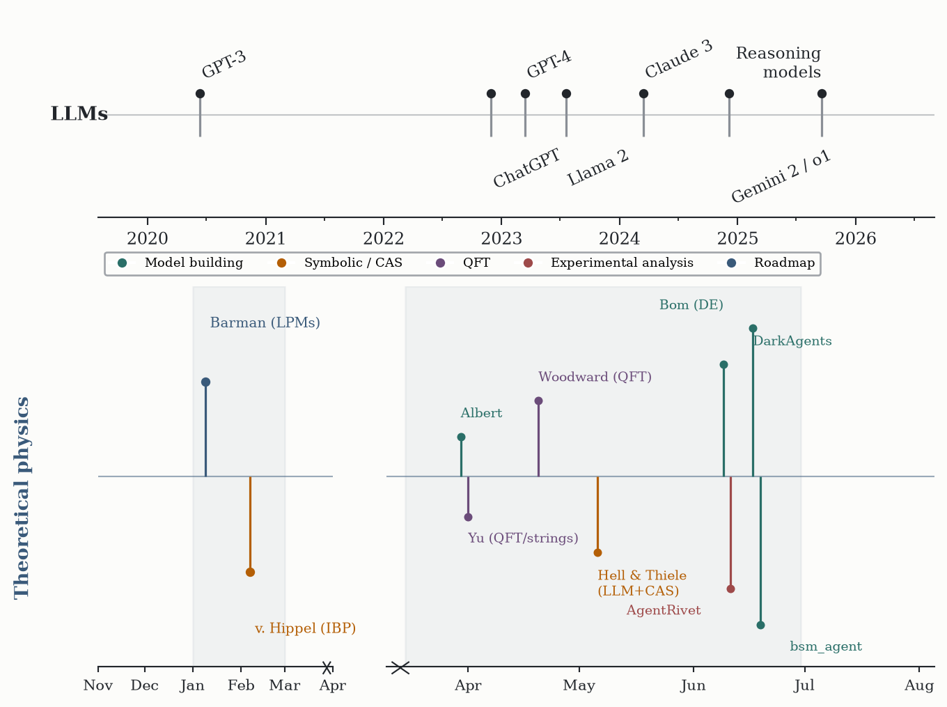
Figure 1: Timeline of LLM milestones (top) and theoretical-physics works that adopt them (bottom). The bottom axis uses a break: 2025 events on the left, the dense March–June 2026 cluster enlarged on the right.

Model building and phenomenology pipelines

bsm_agent (Saad 2026) is perhaps the cleanest example of the pattern described above. The user specifies, in natural language, the quantum numbers of new scalar or fermionic particles. An LLM interprets that specification, resolves ambiguities through confirmation steps, and triggers a deterministic symbolic backend — written in Python, with no LLM involvement — that builds the renormalizable Lagrangian, checks gauge anomalies, expands operators into component fields, derives the electroweak symmetry-breaking stationary conditions, and computes tree-level mass matrices. The LLM is the orchestrator; the correct physics is guaranteed by the symbolic code.¹

DarkAgents (Lucente et al. 2026) applies a similar multi-agent scheme to the domain of astroparticle physics. The system builds complete pipelines: it starts from a classically scale-invariant model, computes first-order cosmological phase transitions, and fits the resulting gravitational-wave spectrum to NANOGrav data. What sets it apart is that DarkAgents also produces an audit report of the assumptions and priors entering each stage — a layer of transparency that hand calculations rarely document with this level of systematicity. In its tests, the system identified inconsistencies in previously published fits and produced new ones using dissipative bulk-flow GW templates. The code is publicly available.²

LLM + computer algebra system

One of the most concrete and least spectacular — in the best sense — results is that of Hell and Thiele (Hell and Thiele 2026). They couple Claude (a frontier commercial LLM) with Maple (a computer algebra system) and evaluate whether the system solves algorithmic tasks in theoretical physics: cosmological perturbations in modified theories of gravity. The LLM receives worked examples as context (in-context learning) and is then asked to solve analogous problems using Maple as a runtime. The finding is measured but significant: with enough worked examples, the system solves most test problems. Typical errors are not computational (Maple guarantees that) but formal: misinterpreting a convention, applying a template where it does not belong.

The pattern is the same: the LLM does not derive; the LLM translates intent into the language of the tool that does.

Feynman-integral reduction

Integration-by-parts (IBP) reduction of Feynman integrals is one of the most well-known computational bottlenecks in high-energy theoretical physics and gravitational-wave physics. The efficiency of the reduction depends critically on heuristics for selecting which IBP identities to use first — a combinatorial optimization problem traditionally solved with handcrafted criteria.

von Hippel and Wilhelm (Hippel and Wilhelm 2025) attacked this problem using funsearch, a genetic-programming variant that generates code via an LLM. The system explores the space of possible heuristics, evaluates each against reduction benchmarks, and evolves the best ones. The authors report that the method rediscovered the state-of-the-art heuristics recently incorporated into IBP solvers and in one case found a small improvement over the state of the art. Again: the LLM does not derive integrals; it generates heuristic candidates that a deterministic solver evaluates.

Autonomous theory-space exploration

Albert (Alexander et al. 2026) deserves separate mention, although its architecture departs from the “LLM as bridge to tools” pattern. It is a neuro-symbolic framework that encodes particle physics as a formal language — symmetries, particles, interactions — with a rule-based grammar. This eliminates hallucinations: the model generates tokenized sequences that are syntactically valid by construction. A reinforcement-learning environment enforces first-principle theoretical constraints, computes observables with radiative corrections, and evaluates statistical likelihood (\(\chi^2\)) against experimental data. Trained only on LEP data — which contain no direct evidence for the top quark — Albert rediscovered the Standard Model and autonomously inferred the necessity and properties of the top quark, predicting its mass at \(178.9 \pm 5.0\ \text{GeV}\), consistent with the modern LHC measurement.

This work is relevant not because it uses an LLM — it does not, in the conventional sense; it is a transformer trained for a specific task — but because it shows that the BSM theory space, whose combinatorial explosion is the standard argument against systematic exploration, can be navigated with modern architectures as long as physical constraints are imposed as part of the environment, not as part of the generative model.

From papers to analysis code

One of the chronic problems of collider phenomenology is the gap between what an ATLAS or CMS paper reports and the code that allows a new model to be compared against that measurement. The Rivet system preserves experimental analyses as C++ routines that any Monte Carlo generator can invoke, but coverage is incomplete: only 39% of measurements have a public, documented routine.

AgentRivet (Costa et al. 2026) uses a multi-stage workflow with commercial LLMs (OpenAI, Anthropic, Google) to extract the analysis information from a published paper and write the missing Rivet routine, with intermediate code and physics reviews as autonomous quality control. The results are encouraging but nuanced: the routines compile with few syntax errors and the physics fidelity is reasonable, but most implementation errors stem from subtle ambiguities in the publication itself — not from LLM failures. That is, the system is only as good as the clarity of the paper it processes.

Language models fine-tuned for QFT

In a more exploratory spirit, Woodward et al. (Woodward et al. 2026) carried out the first academic fine-tuning study of small reasoning models (7B parameters) dedicated specifically to quantum field theory. They generated over 2,500 synthetic problems and curated human-authored problems from arXiv and standard pedagogical resources. They trained with RL and SFT, and release the data, the pipeline, and ~200M tokens of reasoning traces. The work is valuable above all for what it reveals about the process: reasoning errors do not disappear with fine-tuning; they change character, and generalization to other physics domains is limited.

Two complementary benchmarking works help calibrate expectations. Yu et al. (Yu et al. 2026) built a small expert-curated question set in QFT and string theory and found that current LLMs approach ceiling performance on explicit derivations within stable conceptual frames, but systematically degrade when the task requires reconstructing omitted reasoning steps or reorganizing representations under global consistency constraints.

The roadmap: Large Physics Models

I close with an article that reports no concrete system but articulates a vision. Barman et al. (Barman et al. 2025) — a large group with authors from particle physics, computer science, and philosophy of science — proposed the concept of Large Physics Models (LPMs): foundation models specific to physics, integrated with symbolic reasoning modules, experimental data analysis, and literature synthesis. The article, published in European Physical Journal C, organizes the discussion into three pillars — Development, Evaluation, and Philosophical Reflection — and proposes an interdisciplinary collaboration structure inspired by experimental particle-physics collaborations.

What all of this means

The common thread of the works above is not “LLMs solve theoretical physics.” It is more specific and, I think, more interesting: LLMs are turning tools that already existed but were difficult to use into tools accessible via natural language. The pattern repeats:

• bsm_agent: natural language \(\to\) symbolic backend.
• DarkAgents: natural language \(\to\) compute pipeline + audit.
• Hell & Thiele: natural language + examples \(\to\) Maple code.
• funsearch + IBP: natural language (via code generation) \(\to\) heuristics evaluated by solver.
• AgentRivet: published paper \(\to\) Rivet routine.

In each case, the correct physics is guaranteed by a deterministic layer external to the LLM. The LLM solves the interface problem.

This has practical implications. The community does not need, for now, a model that derives on its own — it probably wouldn’t be trustworthy even if it existed. What is needed is investment in documentation, APIs, and wrappers that make existing tools accessible to an LLM, because the LLM already knows — in the statistical sense — how to use them. A SARAH with a well-designed API and machine-readable documentation would be immediately more useful, via LLM, than a SARAH without any of that but coupled to a larger generative model.

But lowering the technical barrier is not enough if physicists cannot cross the one that is already low. To the extent that LLMs turn natural language into tool invocations, the next bottleneck is not the interface — it is the user’s ability to read, audit, and correct what the model produces. Theoretical-physics training should include, in the near future, basic software skills: reading source code, version control, debugging symbolic packages. Not to turn physicists into programmers, but so that verification — which remains the central step of the craft — does not depend on a skill set that most theory PhDs do not receive today.

As theoretical physics evolves and new tools, methods, or theories emerge, building a deterministic layer external to the LLM — one that guarantees the correct application of the physics — will be the most important part for the community to reliably harness LLMs.

What is missing

I end with three directions that this survey leaves open and that probably deserve their own entries in this log:

1. A concrete case study. Take one of the patterns above and run it end-to-end on a real BSM model (with unpublished details withheld), measuring time saved and errors encountered.
2. Operational comparison between models. All the cited works treat “the LLM” as an interchangeable black box. The reality is that different models fail in different ways, and characterizing that for theoretical-physics tasks is a pending contribution.
3. The verification problem. Almost all the systems described delegate correctness to a deterministic layer. But what happens when the deterministic layer does not exist or is itself hard to verify? That is the hardest use case, and it is only beginning to be explored.

References

Alexander, Stephon, Benjamin Bradley, Loukas Gouskos, and Cooper Niu. 2026. “Autonomous Discovery of Particle Physics Theories from Experimental Data.” arXiv Preprint. https://arxiv.org/abs/2603.28935.

Barman, Kristian G., Sascha Caron, Emily Sullivan, et al. 2025. “Large Physics Models: Towards a Collaborative Approach with Large Language Models and Foundation Models.” Eur. Phys. J. C 85: 1066. https://doi.org/10.1140/epjc/s10052-025-14707-8.

Costa, Antonio J., Caterina Doglioni, Christian Gütschow, Andrew D. Pilkington, and Sukanya Sinha. 2026. “AgentRivet: An Automated System for Producing Rivet Routines from Journal Publications.” arXiv Preprint. https://arxiv.org/abs/2606.13535.

Hell, Anamaria, and Leander Thiele. 2026. “LLMs with in-Context Learning for Algorithmic Theoretical Physics.” arXiv Preprint. https://arxiv.org/abs/2605.08212.

Hippel, Matt von, and Matthias Wilhelm. 2025. “Refining Integration-by-Parts Reduction of Feynman Integrals with Machine Learning.” arXiv Preprint. https://arxiv.org/abs/2502.05121.

Lucente, Michele, Silvia Pascoli, Filippo Sala, and Matteo Zandi. 2026. “DarkAgents.” arXiv Preprint. https://arxiv.org/abs/2606.11157.

Saad, Shaikh. 2026. “Large Language Model-Assisted Framework for BSM Model Building.” arXiv Preprint. https://arxiv.org/abs/2606.21316.

Woodward, Nathaniel S., Zhiqi Gao, Yurii Kvasiuk, Kendrick M. Smith, Frederic Sala, and Moritz Münchmeyer. 2026. “Fine-Tuning Small Reasoning Models for Quantum Field Theory.” arXiv Preprint. https://arxiv.org/abs/2604.18936.

Yu, Xingyang, Yinghuan Zhang, Yufei Zhang, and Zijun Cui. 2026. “Grading the Unspoken: Evaluating Tacit Reasoning in Quantum Field Theory and String Theory with LLMs.” arXiv Preprint. https://arxiv.org/abs/2604.14188.

Footnotes

1. github.com/saad-hep/bsm_agent.

2. github.com/PhysicsZandi/DarkAgents.