How to compute a particle decay

For a student who has met Feynman rules and Dirac spinors, but has never carried a decay calculation all the way to a number.

A particle decays. What we measure is how fast: a lifetime, or equivalently a width \(\Gamma\), and the fractions that go into each final state. What theory provides is a Lagrangian. This notebook is the bridge between the two.

We will do the calculation the way you would on paper — spin sums, Dirac traces, phase space — using feynlag to carry the algebra rather than to hide it. Only once we have built a width from scratch will we reach for the machine that does it in one line.

Roadmap

1. Widths, lifetimes and branching ratios

2. The master formula

3. Two-body phase space

4. From a Feynman rule to an amplitude

5. Squaring: why spin sums become traces

6. Trace theorems, hands-on

7. \(h \to \tau\tau\) and the \(\beta^3\) threshold

8. Polarisation sums: \(Z \to \ell\ell\) and \(W \to \ell\nu\)

9. Chirality: why V−A gives exactly half

10. The whole Standard Model at once

11. Off-shell decays: reopening the closed channel

12. Loop-induced decays and the complete Higgs picture

13. Two ways to get it silently wrong

14. Your own model: a \(Z'\)

15. Recap

import sympy as sp
import numpy as np
import matplotlib.pyplot as plt

from feynlag import *
from feynlag.pheno import (
    DecayCalculator, DiracParticle, TwoBodyKinematics, collect_decay_vertices,
    ffs_squared, ffv_squared, kallen, scalar_offshell_vv_width,
    higgs_gammagamma_width, higgs_gg_width, higgs_zgamma_width,
    scalar_vv_s12_integral, two_body_momentum, two_body_phase_space,
    vvs_squared,
)
from feynlag.pheno.lorentz import contract_to_dots, dirac_trace, index, slashed

sp.init_printing()

Missing colon in file PosixPath('/home/moises/.config/matplotlib/stylelib/ifunam.mplstyle'), line 28 ("    '003DA5',")

Missing colon in file PosixPath('/home/moises/.config/matplotlib/stylelib/ifunam.mplstyle'), line 29 ("    'C0392B',")

Missing colon in file PosixPath('/home/moises/.config/matplotlib/stylelib/ifunam.mplstyle'), line 30 ("    '1A6B3A',")

Missing colon in file PosixPath('/home/moises/.config/matplotlib/stylelib/ifunam.mplstyle'), line 31 ("    'FFBE00',")

Missing colon in file PosixPath('/home/moises/.config/matplotlib/stylelib/ifunam.mplstyle'), line 32 ("    '3F6FD1',")

Missing colon in file PosixPath('/home/moises/.config/matplotlib/stylelib/ifunam.mplstyle'), line 33 ("    '8E44AD',")

Missing colon in file PosixPath('/home/moises/.config/matplotlib/stylelib/ifunam.mplstyle'), line 34 ("    'E67E22',")

Missing colon in file PosixPath('/home/moises/.config/matplotlib/stylelib/ifunam.mplstyle'), line 35 ("    '17A589',")

Missing colon in file PosixPath('/home/moises/.config/matplotlib/stylelib/ifunam.mplstyle'), line 36 ("    '2C3E50',")

Missing colon in file PosixPath('/home/moises/.config/matplotlib/stylelib/ifunam.mplstyle'), line 37 ("    'CB4335'])")

Bad value in file PosixPath('/home/moises/.config/matplotlib/stylelib/ifunam.mplstyle'), line 21 ('axes.edgecolor    : #4A4A6A'): Key axes.edgecolor: '' does not look like a color arg

Bad value in file PosixPath('/home/moises/.config/matplotlib/stylelib/ifunam.mplstyle'), line 27 ("axes.prop_cycle : cycler('color', ["): Key axes.prop_cycle: "cycler('color', [" is not a valid cycler construction: Could not parse "cycler('color', [": '[' was never closed (<unknown>, line 1)

Bad value in file PosixPath('/home/moises/.config/matplotlib/stylelib/ifunam.mplstyle'), line 95 ('patch.edgecolor       : face'): Key patch.edgecolor: 'face' does not look like a color arg

1. Widths, lifetimes and branching ratios

An unstable particle has a survival probability that falls exponentially, \(P(t) = e^{-\Gamma t}\). The constant \(\Gamma\) is the decay width, and it is just an inverse lifetime,

\[\tau = \frac{\hbar}{\Gamma}.\]

Because we work in natural units, \(\Gamma\) carries units of energy — quoted in GeV, even though it describes a time.

If several final states are available, each has its own partial width \(\Gamma_i\). They simply add, and the fraction going into channel \(i\) is the branching ratio

\[\mathrm{BR}_i = \frac{\Gamma_i}{\Gamma_\text{tot}}, \qquad \Gamma_\text{tot} = \sum_i \Gamma_i, \qquad \sum_i \mathrm{BR}_i = 1.\]

The \(Z\) boson makes this concrete.

hbar = 6.582119569e-25          # GeV*s
Gamma_Z = 2.4952                # GeV, PDG total width

print(f"Gamma(Z) = {Gamma_Z} GeV")
print(f"tau(Z)   = {hbar / Gamma_Z:.3e} s")

Gamma(Z) = 2.4952 GeV
tau(Z)   = 2.638e-25 s

Around \(2.6\times10^{-25}\) s. That is the number we are going to compute — starting from nothing but a Lagrangian.

2. The master formula

Fermi’s golden rule says a transition rate is (matrix element)² × (density of final states). Made relativistic and specialised to one particle of mass \(M\) decaying at rest, it reads

\[\boxed{\;\Gamma = \frac{1}{2M}\int \overline{|\mathcal{M}|^2}\;\mathrm{d}\Phi_n\;}\]

Three pieces, and we will take them one at a time:

• \(1/2M\) — relativistic normalisation of the decaying state.

• \(\mathrm{d}\Phi_n\) — phase space: how much room the final state has. Pure kinematics; no dynamics at all (§3).

• \(\overline{|\mathcal{M}|^2}\) — the squared amplitude, where all the physics lives (§4–§9).

The bar is not decoration. Real experiments do not prepare or measure spin here, so we

• sum over final-state spins and polarisations (we do not care which one we got),

• average over the decaying particle’s, dividing by its \(2s+1\) states — \(1\) for a scalar, \(3\) for a massive vector.

Getting that factor of 3 wrong for a vector is one of the most common slips.

3. Two-body phase space

For a two-body final state the integral collapses to something you can write down. In the rest frame the two daughters come out back to back with equal and opposite momenta, so once you fix their common magnitude \(|k|\) there is nothing left to integrate but an overall solid angle.

Energy conservation fixes \(|k|\) through the Källén triangle function

\[\lambda(x,y,z) = x^2+y^2+z^2-2xy-2yz-2zx, \qquad |k| = \frac{\sqrt{\lambda(M^2,m_1^2,m_2^2)}}{2M},\]

and the whole phase-space factor becomes

\[\int\mathrm{d}\Phi_2 \;\longrightarrow\; \frac{\sqrt{\lambda(M^2,m_1^2,m_2^2)}}{16\pi M^3}\, \quad\text{(after the }1/2M\text{)}.\]

M, m1, m2 = sp.symbols('M m_1 m_2', positive=True)

kin = TwoBodyKinematics(M, m1, m2)

print("Kallen lambda(M^2, m1^2, m2^2):")
display(sp.factor(kallen(M**2, m1**2, m2**2)))

print("\ndaughter momentum |k|:")
display(two_body_momentum(M, m1, m2))

print("\nthe full phase-space factor sqrt(lambda)/(16 pi M^3):")
display(kin.phase_space())

Kallen lambda(M^2, m1^2, m2^2):

daughter momentum |k|:

the full phase-space factor sqrt(lambda)/(16 pi M^3):

Note the factorised form of \(\lambda\): it contains \(\big(M-(m_1+m_2)\big)\). The moment \(M\) drops below \(m_1+m_2\) that factor changes sign, \(\sqrt\lambda\) becomes imaginary and the decay is closed. Watch this happen.

# equal-mass daughters: how much room is left as they get heavier?
x = np.linspace(0.0, 0.5, 400)                  # x = m/M
ps = np.sqrt(np.clip(1 - 4*x**2, 0, None))      # sqrt(lambda)/M^2 for m1 = m2 = m

fig, ax = plt.subplots(figsize=(6.4, 4.0))
ax.plot(x, ps, lw=2, color='#1f77b4')
ax.axvline(0.5, ls='--', color='0.4')
ax.text(0.492, 0.55, 'threshold  $m = M/2$', rotation=90,
        ha='right', va='center', color='0.3')
ax.set_xlabel(r'daughter mass  $m/M$')
ax.set_ylabel(r'phase space  $\sqrt{\lambda}/M^2$')
ax.set_title('Two-body phase space closes at threshold')
ax.set_xlim(0, 0.52); ax.set_ylim(0, 1.05)
ax.grid(alpha=0.3)
plt.tight_layout()
plt.show()

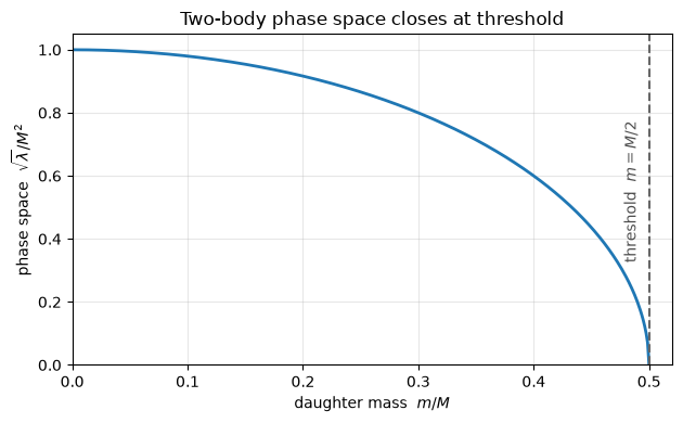
The curve reaches zero at \(m = M/2\) with a vertical tangent — the square root. This is pure kinematics: we have not said one word about the interaction. Any decay, of any particle, through any force, is switched off by this factor as the daughters get heavy enough. Dynamics can only change how fast the curve falls, never that it falls.

4. From a Feynman rule to an amplitude

Now the dynamics. feynlag reads vertices straight off a Lagrangian — that is what the other tutorials in this series do. Let us build the electroweak Standard Model with one lepton generation and simply ask it for its vertices.

(The build is condensed here; SM_Feynman_Rules_Tutorial.ipynb walks it stage by stage.)

GW, G1, VEV, MH = 0.6535, 0.3580, 246.0, 125.25
MZ, MW, MTAU = 91.1876, 80.377, 1.77686

# The electroweak scaffold — gauge groups, Higgs, potential and the
# physical-basis rotations — comes ready-made from feynlag.models. (The
# SM_Feynman_Rules_Tutorial builds all of this by hand, stage by stage.)
ew = electroweak_scaffold(gw=GW, g1=G1, v=VEV, mh=MH)
SU2L, U1Y, H = ew.SU2L, ew.U1Y, ew.H
gw, g1, v = ew.gw, ew.g1, ew.v          # convenience aliases for later cells
ytau = ExternalParameter("ytau", sp.sqrt(2) * MTAU / VEV, positive=True)

# the one piece of physics that IS the point here: a tau lepton + its Yukawa
Ll = WeylFermion("Ll", reps={SU2L: 2, U1Y: -sp.Rational(1, 2)}, chirality="L",
                 nflavors=1, component_names=["nuL", "tauL"])
tauR = WeylFermion("tauR", reps={U1Y: -1}, chirality="R", nflavors=1,
                   component_names=["tauR"])

i = sp.Symbol("i", integer=True)
L = Lagrangian()
ew.add_higgs(L)                                    # kinetic + potential
L.add(fermion_gauge_current(Ll, i) + fermion_gauge_current(tauR, i), sector="gauge")

nuLb, tauLb = Ll.bar_components
nuL, tauL = Ll.components
tauRb, tauRc = tauR.bar_components[0], tauR.components[0]
yuk = -ytau.s * (Bilinear(nuLb[i], diracPR, tauRc[i]) * H.components[0]
                 + Bilinear(tauLb[i], diracPR, tauRc[i]) * H.components[1])
L.add(yuk + sp.conjugate(yuk), sector="yukawa")

model = Model("SM_lepton", gauge_groups=ew.gauge_groups,
              fields=ew.fields + [Ll, tauR],
              parameters=ew.parameters + [ytau], lagrangian=L)
model.solve_tadpoles([ew.mu2])

# physical basis: the standard Weinberg + W± rotations, in one call
phys = to_physical_basis(model, ew)
Z, A, Wp, Wm, h, G0, Gp, Gm = (phys.Z, phys.A, phys.Wp, phys.Wm,
                               phys.h, phys.G0, phys.Gp, phys.Gm)
cmap, bosons = phys.cmap, phys.bosons

# a Dirac fermion is two Weyl fields in feynlag: say which legs are one particle
tau, taubar, nutau, nutaubar = sp.symbols("tau taubar nu_tau nu_taubar")
particle_map = {tauL[i]: tau, tauRc[i]: tau, tauLb[i]: taubar, tauRb[i]: taubar,
                nuL[i]: nutau, nuLb[i]: nutaubar}
print("model built")

model built

Every fermion vertex feynlag produces has the same shape,

\[\Gamma \;=\; g_L P_L + g_R P_R \qquad\text{or}\qquad \Gamma^\mu \;=\; \gamma^\mu\,(g_L P_L + g_R P_R),\]

a scalar sandwich or a vector current, each with a left- and a right-handed coupling. So a vertex is fully specified by the pair \((g_L, g_R)\). Here they are for the \(Z\) and the Higgs:

vertices = collect_decay_vertices(model, bosons, fermion_sectors=("gauge", "yukawa"),
                                  conjugate_map=cmap, particle_map=particle_map)

for vtx in vertices:
    if vtx.vertex_type in ("FFV", "FFS") and (Z in vtx.particles or h in vtx.particles):
        legs = " ".join(str(p) for p in vtx.particles)
        print(f"{vtx.vertex_type}  {legs}")
        print(f"      g_L = {sp.factor(sp.expand(vtx.g_left))}")
        print(f"      g_R = {sp.factor(sp.expand(vtx.g_right))}")

FFV  taubar tau Z
      g_L = I*(g1 - gw)*(g1 + gw)/(2*sqrt(g1**2 + gw**2))
      g_R = I*g1**2/sqrt(g1**2 + gw**2)
FFV  nu_taubar nu_tau Z
      g_L = I*sqrt(g1**2 + gw**2)/2
      g_R = 0
FFS  taubar tau H0_r
      g_L = -sqrt(2)*I*ytau/2
      g_R = -sqrt(2)*I*ytau/2

Read these off against what you know:

• \(Z\tau\tau\) has \(g_L \ne g_R\) — the weak interaction is chiral.

• \(Z\nu\nu\) has \(g_R = 0\) exactly. There is no right-handed neutrino to couple to.

• \(h\tau\tau\) has \(g_L = g_R = -i\,y_\tau/\sqrt2 = -i\,m_\tau/v\) — the Higgs is not chiral, and it couples in proportion to mass.

(The factors of \(i\) are the Feynman-rule \(i\); they cancel when we square.)

5. Squaring: why spin sums become traces

The amplitude for a scalar decaying to a fermion pair is

\[\mathcal{M} = \bar u(p_1)\,\Gamma\, v(p_2),\]

a single complex number once the spinors are fixed. We need \(|\mathcal{M}|^2\) summed over the final spins. Using \(\mathcal{M}^* = \bar v(p_2)\,\bar\Gamma\, u(p_1)\) with \(\bar\Gamma = \gamma^0\Gamma^\dagger\gamma^0\),

\[\sum_\text{spins}|\mathcal{M}|^2 = \sum_{s_1,s_2}\bar u(p_1)\Gamma v(p_2)\,\bar v(p_2)\bar\Gamma u(p_1).\]

Now the key step. The completeness relations

\[\sum_s u(p)\bar u(p) = \not p + m, \qquad \sum_s v(p)\bar v(p) = \not p - m\]

replace each spinor pair by a \(4\times4\) matrix. What is left is a product of matrices sandwiched between \(\bar u \dots u\) with the same index summed at both ends — which is by definition a trace:

\[\boxed{\;\sum_\text{spins}|\mathcal{M}|^2 = \mathrm{Tr}\big[(\not p_1 + m_1)\,\Gamma\,(\not p_2 - m_2)\,\bar\Gamma\big]\;}\]

This is why every decay calculation in the textbooks turns into trace algebra. The spins are gone; only momenta and masses remain.

mu, nu = index('mu'), index('nu')
p1, p2 = kin.p1, kin.p2

# the spin sums themselves
print("sum u ubar = p1_slash + m1 :", slashed(p1, mu) + m1)
print("sum v vbar = p2_slash - m2 :", slashed(p2, nu) - m2)

sum u ubar = p1_slash + m1 : m_1 + p1(L_0)*GammaMatrix(-L_0)
sum v vbar = p2_slash - m2 : -m_2 + p2(L_0)*GammaMatrix(-L_0)

6. Trace theorems, hands-on

Four facts do almost all the work:

\[\mathrm{Tr}[\text{odd number of }\gamma] = 0, \qquad \mathrm{Tr}[\gamma^\mu\gamma^\nu] = 4g^{\mu\nu},\]

\[\mathrm{Tr}[\gamma^\mu\gamma^\nu\gamma^\rho\gamma^\sigma] = 4\left(g^{\mu\nu}g^{\rho\sigma} - g^{\mu\rho}g^{\nu\sigma} + g^{\mu\sigma}g^{\nu\rho}\right), \qquad \mathrm{Tr}[P_{L,R}] = 2.\]

The first one is why mass terms and momentum terms never mix: each \(\not p\) brings one \(\gamma\), so a term with an odd number of them dies.

Let us evaluate the simplest non-trivial trace, \(\mathrm{Tr}[\not p_1 \not p_2]\), in the two steps you would do by hand.

chain = slashed(p1, mu) * slashed(p2, nu)

step1 = dirac_trace(chain)
print("step 1 -- apply Tr[gamma^mu gamma^nu] = 4 g^{mu nu}:")
print("   ", step1, "     i.e.  4 p1.p2")

step 1 -- apply Tr[gamma^mu gamma^nu] = 4 g^{mu nu}:
    4*p1(L_0)*p2(-L_0)      i.e.  4 p1.p2

The result is still written with an abstract contracted index. The second step puts the momenta on shell — a two-body final state has only three independent invariants, and all of them are fixed by the masses:

\[p_1^2 = m_1^2, \qquad p_2^2 = m_2^2, \qquad p_1\!\cdot\! p_2 = \frac{M^2 - m_1^2 - m_2^2}{2},\]

the last from squaring \(M^2 = (p_1+p_2)^2\).

print("on-shell dot products:")
print("   p1.p1 =", kin.dot(p1, p1))
print("   p2.p2 =", kin.dot(p2, p2))
print("   p1.p2 =", kin.dot(p1, p2))

step2 = contract_to_dots(step1, kin.dot)
print("\nstep 2 -- substitute them:")
print("   Tr[p1_slash p2_slash] =", sp.expand(step2))

on-shell dot products:
   p1.p1 = m_1**2
   p2.p2 = m_2**2
   p1.p2 = M**2/2 - m_1**2/2 - m_2**2/2

step 2 -- substitute them:
   Tr[p1_slash p2_slash] = 2*M**2 - 2*m_1**2 - 2*m_2**2

So \(\mathrm{Tr}[\not p_1\not p_2] = 4\,p_1\!\cdot\!p_2 = 2M^2 - 2m_1^2 - 2m_2^2\): a plain function of the masses. Every squared amplitude below is built from exactly these two steps.

7. \(h \to \tau\tau\) and the \(\beta^3\) threshold

Assemble the scalar case. With \(\Gamma = g_LP_L + g_RP_R\) the conjugate is \(\bar\Gamma = \bar g_L P_R + \bar g_R P_L\) (bare projectors swap under \(\gamma^0(\cdot)^\dagger\gamma^0\)), and pushing projectors through with \(P_{L,R}\not p = \not p P_{R,L}\), \(P_LP_R = 0\) splits the trace cleanly in two:

• the chirality-diagonal terms keep the momenta and lose the masses,

• the chirality-mixing terms keep \(m_1m_2\) and lose the momenta.

\[\sum|\mathcal{M}|^2 = 2(|g_L|^2+|g_R|^2)\,(p_1\!\cdot\!p_2) - 4\,m_1m_2\,\mathrm{Re}(g_L\bar g_R).\]

gL, gR = sp.symbols('g_L g_R', real=True)
mh, mf = sp.symbols('m_h m_f', positive=True)

kin_h = TwoBodyKinematics(mh, mf, mf)
amp2 = ffs_squared(gL, gR, kin_h)
print("summed |M|^2 for S -> f fbar:")
display(sp.factor(sp.expand(amp2)))

summed |M|^2 for S -> f fbar:

# the Higgs is not chiral: g_L = g_R = m_f/v
vv = sp.Symbol('v', positive=True)
width_h = sp.simplify(ffs_squared(mf/vv, mf/vv, kin_h) * kin_h.phase_space())
display(sp.factor(width_h))

beta = sp.sqrt(1 - 4*mf**2/mh**2)
expected = mh * mf**2 * beta**3 / (8*sp.pi*vv**2)
print("matches  m_h m_f^2 beta^3 / (8 pi v^2)?",
      sp.simplify(sp.expand(width_h - expected)) == 0)

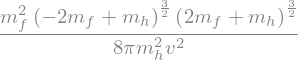
matches  m_h m_f^2 beta^3 / (8 pi v^2)? True

\[\Gamma(h\to f\bar f) = \frac{N_c\, m_h\, m_f^2\,\beta^3}{8\pi v^2}, \qquad \beta = \sqrt{1 - 4m_f^2/m_h^2}.\]

Two things to notice.

\(\Gamma \propto m_f^2\). The Higgs couples proportionally to mass, so it decays preferentially to the heaviest thing it can reach. That single fact drives the entire Higgs search programme.

\(\beta^3\), not \(\beta\). One power of \(\beta\) is the phase space from §3. The other two come from the dynamics: a CP-even scalar decaying to a fermion pair produces them in a P-wave (\(\ell=1\)), and an \(\ell\)-wave amplitude is suppressed by \(\beta^{\ell}\) near threshold — \(\beta^{2\ell}\) in the rate. A CP-odd scalar decays S-wave and would give plain \(\beta\).

b = np.linspace(0, 1, 400)

fig, ax = plt.subplots(figsize=(6.4, 4.0))
ax.plot(b, b**3, lw=2, color='#1f77b4', label=r'CP-even (P-wave):  $\beta^3$')
ax.plot(b, b, lw=2, color='#d62728', ls='-.', label=r'CP-odd (S-wave):  $\beta^1$')
ax.set_xlabel(r'velocity  $\beta=\sqrt{1-4m_f^2/m_h^2}$   (0 = threshold)')
ax.set_ylabel(r'$\Gamma$ / (its $\beta\!\to\!1$ value)')
ax.set_title('Near threshold the CP of the parent is visible in the lineshape')
ax.legend()
ax.grid(alpha=0.3)
ax.set_xlim(0, 1); ax.set_ylim(0, 1.02)
plt.tight_layout()
plt.show()

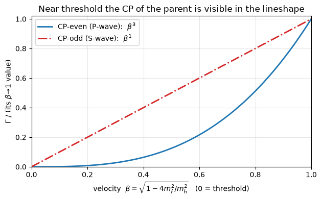
Right at threshold (\(\beta\to0\)) the CP-even curve leaves the axis much more slowly. This is not an academic distinction: the shape of a threshold turn-on is one of the ways the spin and CP of a new particle get pinned down experimentally.

8. Polarisation sums: \(Z\to\ell\ell\) and \(W\to\ell\nu\)

A decaying vector brings two changes. Its amplitude carries a polarisation vector, \(\mathcal{M} = \epsilon_\mu \bar u\,\Gamma^\mu v\), so squaring needs the polarisation sum

\[\sum_\text{pol}\epsilon_a\epsilon^*_b = -g_{ab} + \frac{P_aP_b}{M^2},\]

and because a massive vector has three states we must average, dividing by 3. Everything else is the same trace algebra.

mZ = sp.Symbol('m_Z', positive=True)
m = sp.Symbol('m', positive=True)

kin_Z = TwoBodyKinematics(mZ, m, m)
width_V = sp.simplify(ffv_squared(gL, gR, kin_Z) * kin_Z.phase_space())

betaZ = sp.sqrt(1 - 4*m**2/mZ**2)
closed = (mZ*betaZ/(24*sp.pi)) * ((gL**2 + gR**2)*(1 - m**2/mZ**2)
                                  + 6*gL*gR*m**2/mZ**2)
print("matches the closed form?", sp.simplify(sp.expand(width_V - closed)) == 0)
display(sp.factor(width_V))

matches the closed form? True

\[\Gamma(V\to f\bar f) = \frac{M\beta}{24\pi} \left[(g_L^2+g_R^2)\Big(1-\frac{m^2}{M^2}\Big) + 6\,g_Lg_R\frac{m^2}{M^2}\right].\]

Note the \(g_Lg_R\) term: it needs both chiralities and a mass. It is the piece that will bite us in §13.

Now put in the Standard Model’s own couplings and compare with the PDG.

g, gp = gw.s, g1.s
gZ = sp.sqrt(g**2 + gp**2)

# SM neutral-current couplings (massless limit for the leptons)
couplings = {
    r'$Z \to \nu\bar\nu$':      (gZ/2, 0),                       # purely left-handed
    r'$Z \to \tau^+\tau^-$':    ((gp**2 - g**2)/(2*gZ), gp**2/gZ),
}
vals = {g: GW, gp: G1}

rows = []
for label, (cl, cr) in couplings.items():
    w = ffv_squared(cl, cr, TwoBodyKinematics(mZ, 0, 0)) * TwoBodyKinematics(mZ, 0, 0).phase_space()
    rows.append((label, float(sp.simplify(w).subs(vals).subs(mZ, MZ))))

for label, w in rows:
    print(f"{label:26s}  Gamma = {w:.4f} GeV")

$Z \to \nu\bar\nu$          Gamma = 0.1679 GeV
$Z \to \tau^+\tau^-$        Gamma = 0.0844 GeV

pdg = {r'$Z \to \nu\bar\nu$': 0.1663, r'$Z \to \tau^+\tau^-$': 0.0841}

labels = [r[0] for r in rows]
ours = [r[1] for r in rows]
theirs = [pdg[l] for l in labels]
y = np.arange(len(labels))

fig, ax = plt.subplots(figsize=(6.8, 3.2))
ax.barh(y - 0.19, ours,   height=0.36, color='#1f77b4', label='this notebook (tree level)')
ax.barh(y + 0.19, theirs, height=0.36, color='#bbbbbb', label='PDG')
ax.set_yticks(y); ax.set_yticklabels(labels)
ax.set_xlabel(r'partial width $\Gamma$  [GeV]')
ax.set_title('Z partial widths, per generation')
ax.set_xlim(0, 0.21)
ax.legend(loc='upper right')
ax.grid(alpha=0.3, axis='x')
plt.tight_layout()
plt.show()

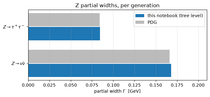
Two tree-level numbers landing within about 1% of experiment — the residual is genuine higher-order physics we have not included.

And note why the invisible channel is the bigger one. The neutrino is purely left-handed, so it gets the full \(g_L^2\) with nothing subtracted; the charged lepton’s left- and right-handed couplings are individually smaller. Chirality is directly visible in the bar chart.

9. Chirality: why V−A gives exactly half

The weak charged current is pure \(V-A\): only \(P_L\). What does that do to a width?

Since \(P_L = \tfrac12(1-\gamma_5)\) and the projector is idempotent, a chiral current keeps exactly half of the vector-current trace. So a \(g_R = 0\) coupling should give precisely half the width of a \(g_L = g_R = g\) one.

gsym, Msym = sp.symbols('g M', positive=True)
kin_m0 = TwoBodyKinematics(Msym, 0, 0)

vector = sp.simplify(ffv_squared(gsym, gsym, kin_m0) * kin_m0.phase_space())
chiral = sp.simplify(ffv_squared(gsym, 0, kin_m0) * kin_m0.phase_space())

print("vector current  g(gamma^mu)        :", vector, "   = g^2 M / 12 pi")
print("chiral current  g(gamma^mu P_L)    :", chiral, "   = g^2 M / 24 pi")
print("exactly half?", sp.simplify(vector - 2*chiral) == 0)

# the W: coupling is g/sqrt(2), purely left-handed
mW = sp.Symbol('m_W', positive=True)
kin_W = TwoBodyKinematics(mW, 0, 0)
width_W = sp.simplify(ffv_squared(gsym/sp.sqrt(2), 0, kin_W) * kin_W.phase_space())
print("\nGamma(W -> l nu) =", width_W, "  = g^2 m_W / 48 pi")
print("numerically      =", float(width_W.subs({gsym: GW, mW: MW})), "GeV   (PDG 0.2264)")

vector current  g(gamma^mu)        : M*g**2/(12*pi)    = g^2 M / 12 pi
chiral current  g(gamma^mu P_L)    : M*g**2/(24*pi)    = g^2 M / 24 pi
exactly half? True

Gamma(W -> l nu) = g**2*m_W/(48*pi)   = g^2 m_W / 48 pi
numerically      = 0.2276312410961552 GeV   (PDG 0.2264)

A word on \(\gamma_5\), because it is where hand calculations go wrong. Writing \(P_L = \tfrac12(1-\gamma_5)\) leaves a term \(\mathrm{Tr}[X\gamma_5]\), which produces the totally antisymmetric \(\epsilon^{\mu\nu\rho\sigma}\).

For a two-body decay that term is always zero, and it is worth seeing why: \(\epsilon\) needs four independent four-vectors to be non-zero, but a 1→2 final state offers only two independent momenta (\(P = p_1+p_2\) is not a third), and any leftover free index gets contracted with the polarisation sum, which is symmetric. Antisymmetric times symmetric vanishes.

That argument fails for a three-body decay — which is exactly why feynlag refuses to drop the term unless it can prove the conditions hold, rather than assuming it.

10. The whole Standard Model at once

Everything so far — vertices, spin sums, traces, phase space, thresholds — is what DecayCalculator automates. Having done it by hand, here is the machine.

You give it the model, a mass for every leg, and the map that says which Weyl legs form one Dirac particle. It finds every three-leg vertex containing the parent and returns a width per channel.

mZs, mWs, mhs, mtaus = sp.symbols("m_Z m_W m_h m_tau", positive=True)
masses = {Z: mZs, Wp: mWs, Wm: mWs, A: 0, h: mhs,
          tau: mtaus, taubar: mtaus, nutau: 0, nutaubar: 0}

calc = DecayCalculator(model, masses, boson_fields=bosons,
                       fermion_sectors=("gauge", "yukawa"),
                       conjugate_map=cmap, particle_map=particle_map,
                       parameters=model.parameters)

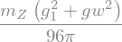
for children, width in calc.partial_widths(Z).items():
    print("Z ->", " ".join(str(c) for c in children))
    display(sp.simplify(width))

Z -> taubar tau

Z -> nu_taubar nu_tau

numbers = {mZs: MZ, mWs: MW, mhs: MH, mtaus: MTAU}

for parent, name in ((Z, 'Z'), (Wp, 'W+'), (h, 'h')):
    widths = calc.numeric_partial_widths(parent, extra=numbers)
    total = sum(widths.values())
    print(f"{name}:")
    for children, w in sorted(widths.items(), key=lambda kv: str(kv[0])):
        kids = " ".join(str(c) for c in children)
        tag = "" if w else "   (closed)"
        print(f"    -> {kids:<16} {w:9.5f} GeV{tag}")
    if total:
        print(f"    lifetime from these channels: {hbar/total:.3e} s")

Z:
    -> nu_taubar nu_tau   0.16787 GeV
    -> taubar tau         0.08424 GeV
    lifetime from these channels: 2.611e-24 s

W+:
    -> nu_taubar tau      0.22746 GeV
    lifetime from these channels: 2.894e-24 s

h:
    -> Wm Wp              0.00000 GeV   (closed)
    -> Z Z                0.00000 GeV   (closed)
    -> taubar tau         0.00026 GeV
    lifetime from these channels: 2.535e-21 s

Compare the \(Z\) line with §1: we started from \(\Gamma_\text{tot}=2.4952\) GeV and a lifetime of \(2.6\times10^{-25}\) s. Our number is longer because we built only one lepton generation and no quarks — the real \(Z\) has many more channels open, so it decays faster. Add them and you converge on the measured value.

The Higgs branching ratios

Nothing stops us from asking what the Higgs would do at a different mass. This reproduces one of the most familiar plots in particle physics.

One practical point, and it is the subject of §13: we cannot call numeric_partial_widths at every point of a fine grid — it re-derives the widths symbolically each time. Instead take each symbolic width once, lambdify it, and apply the threshold condition explicitly.

higgs_widths = calc.partial_widths(h)
param_vals = model.parameters.numeric()

grid = np.linspace(20, 300, 561)
thresholds = {(Wm, Wp): 2*MW, (Z, Z): 2*MZ, (taubar, tau): 2*MTAU}
pretty = {(Wm, Wp): r'$W^+W^-$', (Z, Z): r'$ZZ$', (taubar, tau): r'$\tau^+\tau^-$'}

curves = {}
for key, expr in higgs_widths.items():
    f = sp.lambdify(mhs, expr.subs(param_vals).subs({mZs: MZ, mWs: MW, mtaus: MTAU}),
                    "numpy")
    with np.errstate(invalid='ignore'):
        y = np.where(grid > thresholds[key], f(grid), 0.0)
    curves[key] = np.nan_to_num(y)          # below threshold sqrt(lambda) is imaginary

total = sum(curves.values())
for mtest in (125.25, 170, 200, 300):
    j = int(np.argmin(abs(grid - mtest)))
    br = {pretty[k]: curves[k][j]/total[j] for k in curves}
    print(f"m_h = {mtest:6.2f} GeV   Gamma_tot = {total[j]:8.4f} GeV   " +
          "  ".join(f"BR({n}) = {x:.3f}" for n, x in br.items()))

m_h = 125.25 GeV   Gamma_tot =   0.0003 GeV   BR($W^+W^-$) = 0.000  BR($ZZ$) = 0.000  BR($\tau^+\tau^-$) = 1.000
m_h = 170.00 GeV   Gamma_tot =   0.3711 GeV   BR($W^+W^-$) = 0.999  BR($ZZ$) = 0.000  BR($\tau^+\tau^-$) = 0.001
m_h = 200.00 GeV   Gamma_tot =   1.4227 GeV   BR($W^+W^-$) = 0.734  BR($ZZ$) = 0.266  BR($\tau^+\tau^-$) = 0.000
m_h = 300.00 GeV   Gamma_tot =   8.4429 GeV   BR($W^+W^-$) = 0.688  BR($ZZ$) = 0.312  BR($\tau^+\tau^-$) = 0.000

fig, ax = plt.subplots(figsize=(7.2, 4.4))
colors = {(Wm, Wp): '#1f77b4', (Z, Z): '#d62728', (taubar, tau): '#2ca02c'}
for key in [(taubar, tau), (Wm, Wp), (Z, Z)]:
    ax.plot(grid, curves[key]/np.where(total > 0, total, 1), lw=2,
            color=colors[key], label=pretty[key])

ax.axvline(2*MW, ls='--', color='0.5'); ax.axvline(2*MZ, ls='--', color='0.5')
ax.text(2*MW - 3, 0.55, r'$2m_W$', rotation=90, ha='right', color='0.35')
ax.text(2*MZ + 3, 0.55, r'$2m_Z$', rotation=90, ha='left', color='0.35')
ax.axvline(MH, ls=':', color='#ff7f0e', lw=2)
ax.text(MH - 3, 0.30, 'the real Higgs, 125 GeV', rotation=90, ha='right',
        color='#ff7f0e')

ax.set_xlabel(r'$m_h$  [GeV]')
ax.set_ylabel('branching ratio')
ax.set_title('Higgs branching ratios vs its mass (tree level, this field content)')
ax.set_xlim(20, 300); ax.set_ylim(0, 1.05)
ax.legend(loc='center left'); ax.grid(alpha=0.3)
plt.tight_layout()
plt.show()

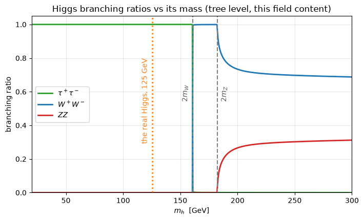
The shape is the physics:

• Below \(2m_W\) only \(\tau\tau\) is open, so it takes everything by default.

• At \(2m_W = 160.8\) GeV the \(WW\) channel opens and immediately dominates — gauge couplings are far larger than a lepton Yukawa.

• At \(2m_Z = 182.4\) GeV \(ZZ\) follows, settling near \(WW\!:\!ZZ \approx 2\!:\!1\) (two charge states of the \(W\), against one \(Z\) that costs an identical-particle \(1/2!\)).

This is the on-shell story: each \(VV\) channel is flat zero until \(2m_V\), so at the physical 125 GeV the plot says \(\tau\tau\) takes essentially everything. Two things close the gap to reality. The fermions we have not declared yet (\(b\bar b\) actually dominates) — next. And the off-shell \(WW^*\): below \(2m_W\) the two-body channel is shut, but the Higgs still reaches a real \(W\) and a virtual one — a three-body decay we compute in §11. (The loop-induced \(\gamma\gamma\) stays out of reach of a tree-level engine — that is Tier 3 of decays_roadmap.md.) The machinery is right; we are still adding content.

The fermions we were missing — one DiracParticle each

The gap above is not a limitation of the machinery — it is missing content. The Higgs couples to every massive fermion, and each \(h\to f\bar f\) is the very \(\beta^3\) scalar decay of §7. All that is missing is declaring those fermions.

Doing that exposes the bookkeeping §13.1 is about to warn you against: each Dirac fermion is two Weyl legs, needs a mass, and — for quarks — a colour factor \(N_c=3\). Tracked as three separate dicts, they drift out of sync. So feynlag bundles them into one object, a DiracParticle:

DiracParticle("b", left=Qb.components[1], right=bR.components[0], mass=mb, color=3)

The bar legs are found automatically (via the bar_partner registry), the mass travels with the particle, and the colour \(N_c\) is applied once — the per-leg double-count that silently inflates a quark width by \(9\times\) (§13.1) is simply unreachable.

# a compact Higgs + fermions model (Higgs sector only; no EW rotations needed
# for h -> f fbar). Running masses at ~m_h, so the branching ratios are realistic.
run = {"tau": 1.777, "mu": 0.1057, "b": 2.79, "c": 0.62, "s": 0.055}
ncol = {"tau": 1, "mu": 1, "b": 3, "c": 3, "s": 3}

gwf = ExternalParameter("gwf", GW, positive=True)
g1f = ExternalParameter("g1f", G1, positive=True)
vf = ExternalParameter("vf", VEV, positive=True, unit_dim=1)
lamf = ExternalParameter("lamf", MH**2 / (2 * VEV**2))
mu2f = InternalParameter("mu2f", unit_dim=2)
SU2f, U1f = SU2("SU2f", coupling=gwf), U1("U1f", coupling=g1f)
Hf = Scalar("Hf", reps={SU2f: 2, U1f: sp.Rational(1, 2)}, component_names=["Gpf", "H0f"])
Hf.expand_vev({Hf.components[1]: vf})
H0f = Hf.components[1]
j = sp.Symbol("j", integer=True)

Lf = Lagrangian()
Lf.add((dag(Dmu(Hf)) * Dmu(Hf))[0], sector="kinetic")
Lf.add(-(-mu2f.s * (dag(Hf) * Hf.mat)[0] + lamf.s * (dag(Hf) * Hf.mat)[0]**2),
       sector="potential")

fields_f, params_f, diracs, ysym = [Hf], [gwf, g1f, vf, lamf, mu2f], [], {}
for name in run:
    Qf = WeylFermion(f"Q{name}", reps={SU2f: 2, U1f: sp.Rational(1, 6)}, chirality="L",
                     nflavors=1, component_names=[f"u{name}", f"d{name}"])
    fR = WeylFermion(f"{name}R", reps={U1f: -sp.Rational(1, 3)}, chirality="R",
                     nflavors=1, component_names=[f"{name}Rc"])
    y = ExternalParameter(f"y_{name}", sp.sqrt(2) * run[name] / VEV, positive=True)
    term = -y.s * Bilinear(Qf.bar_components[1][j], diracPR, fR.components[0][j]) * H0f
    Lf.add(term + sp.conjugate(term), sector="yukawa")
    fields_f += [Qf, fR]; params_f.append(y); ysym[name] = y
    mfs = sp.Symbol(f"m_{name}", positive=True)
    diracs.append((name, DiracParticle(name, left=Qf.components[1],
                                       right=fR.components[0], mass=mfs, color=ncol[name]),
                   mfs, run[name]))

fields_f += [SU2f.bosons("Wf"), U1f.bosons("Bf")]
Hf_model = Model("SM_higgs_ferms", gauge_groups=[SU2f, U1f], fields=fields_f,
                 parameters=params_f, lagrangian=Lf)
Hf_model.solve_tadpoles([mu2f])
hf = sp.Symbol("H0f_r", real=True)
print("full-fermion Higgs model built:", [n for n, *_ in diracs])

full-fermion Higgs model built: ['tau', 'mu', 'b', 'c', 's']

mhf = sp.Symbol("m_hf", positive=True)
calc_f = DecayCalculator(Hf_model, {hf: mhf}, boson_fields=[hf],
                         fermion_sectors=("yukawa",),
                         particles=[dp for _, dp, _, _ in diracs],
                         parameters=Hf_model.parameters)

mass_pt = {mhf: MH}
mass_pt.update({ms: val for _, _, ms, val in diracs})
widths_f = calc_f.numeric_partial_widths(hf, extra=mass_pt)
assert calc_f.unmatched_channels == []          # every fermion is declared

total_f = sum(widths_f.values())
print(f"{'channel':<14}{'Gamma [MeV]':>13}{'BR':>9}")
print("-" * 36)
for children in sorted(widths_f, key=lambda k: -widths_f[k]):
    name = str(children[1])
    print(f"h -> {name}bar {name:<4}{widths_f[children]*1e3:>11.4f}{widths_f[children]/total_f:>9.3f}")
print("-" * 36)
print(f"{'total (fermions)':<14}{total_f*1e3:>13.4f}")

channel         Gamma [MeV]       BR
------------------------------------
h -> bbar b        1.9174    0.843
h -> taubar tau      0.2597    0.114
h -> cbar c        0.0950    0.042
h -> mubar mu       0.0009    0.000
h -> sbar s        0.0007    0.000
------------------------------------
total (fermions)       2.2737

labels = [str(c[1]) for c in sorted(widths_f, key=lambda k: widths_f[k])]
brs = [widths_f[c] / total_f for c in sorted(widths_f, key=lambda k: widths_f[k])]
tex = {"b": r"$b\bar b$", "tau": r"$\tau^+\tau^-$", "c": r"$c\bar c$",
       "mu": r"$\mu^+\mu^-$", "s": r"$s\bar s$"}

fig, ax = plt.subplots(figsize=(6.8, 3.6))
ax.barh(range(len(labels)), brs, color="#1f77b4")
ax.set_yticks(range(len(labels)))
ax.set_yticklabels([tex[l] for l in labels])
ax.set_xlabel("branching ratio (tree-level fermions only)")
ax.set_title(r"Higgs fermionic branching ratios at $m_h=125$ GeV")
for k, b in enumerate(brs):
    ax.text(b + 0.005, k, f"{b:.1%}", va="center", color="0.3")
ax.set_xlim(0, 1.0); ax.grid(alpha=0.3, axis="x")
plt.tight_layout()
plt.show()

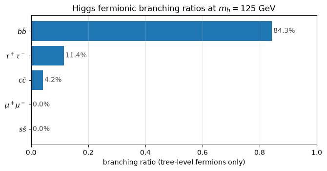
Now \(b\bar b\) dominates — about 84% of the tree-level fermionic width — exactly as the canonical Higgs plot shows, with \(\tau\tau\) a distant second. The two facts from §7 are both visible: the width tracks \(m_f^2\) (so the heavy \(b\) wins), and quarks carry the extra \(N_c=3\).

Every tree-level fermionic channel is now here, declared cleanly — and calc_f.unmatched_channels came back empty, our guarantee that no fermion was silently dropped. What is still missing from the plot is the off-shell \(WW^*/ZZ^*\) — which, it turns out, is not beyond a tree-level engine at all. That is §11.

11. Off-shell decays: reopening the closed channel

Look again at where the Higgs plot said \(WW\) is closed: below \(2m_W = 160.8\) GeV the two-body width is exactly zero, because \(\sqrt{\lambda(m_h^2,m_W^2,m_W^2)}\) is imaginary (§12.2 makes a lesson of this). Yet the measured Higgs, at 125 GeV, decays to \(WW^*\) about a fifth of the time. How?

Because the Higgs does not need two on-shell \(W\)’s. It reaches one on-shell \(W\) and one off-shell \(W^*\) that immediately materialises as a fermion pair:

\[h \;\to\; W\,(W^* \to f\bar f').\]

That is a three-body decay, \(1\to3\), and it is where the machinery takes its one real architectural step. A \(1\to2\) amplitude squares a single vertex. Here the amplitude is vertex × propagator × vertex — the \(hWW\) coupling, the internal \(W^*\) propagator

\[\frac{-i\,(g_{\mu\nu} - q_\mu q_\nu/m_W^2)}{q^2 - m_W^2 + i\,m_W\Gamma_W},\]

and the \(W^*ff'\) current. The propagator’s momentum \(q=p_f+p_{\bar f'}\) flows into the trace algebra — but \(q = p_2+p_3\) is just a sum of the two fermion momenta, so the same covariant engine from §6 contracts it with nothing new to learn.

One tidy detail: below threshold \(q^2\) can never reach \(m_W^2\) (its largest value is \((m_h-m_W)^2 \approx 2000 \ll m_W^2 \approx 6500\)), so the propagator never hits its pole and the width \(\Gamma_W\) in the denominator barely matters. The decay is genuinely off-shell, never resonant.

# the W and Z total widths that feed the Breit-Wigner (themselves decay outputs)
GammaW, GammaZ = 2.085, 2.4952
gZ = np.sqrt(GW**2 + G1**2)
sw2 = G1**2 / (GW**2 + G1**2)

# h -> WW*: hWW = g m_W; 9 fermion channels (3 lepton + 2 quark gen x 3 colour),
# each with the V-A coupling g/sqrt(2); factor 2 for which W is on-shell
gWW = scalar_offshell_vv_width(MH, MW, GammaW, GW * MW,
                               [(GW / np.sqrt(2), 0.0, 9)], identical=False)

# h -> ZZ*: hZZ = g_Z m_Z; real chiral Z->ff couplings; identical Z (no factor 2)
zchan = [(gZ * (T3 - Q * sw2), gZ * (-Q * sw2), Nc * cnt)
         for T3, Q, Nc, cnt in [(0.5, 0, 1, 3), (-0.5, -1, 1, 3),
                                (0.5, 2/3, 3, 2), (-0.5, -1/3, 3, 3)]]
gZZ = scalar_offshell_vv_width(MH, MZ, GammaZ, gZ * MZ, zchan, identical=True)

print(f"Gamma(h -> WW*) = {gWW*1e3:7.4f} MeV   (Keung-Marciano ~0.80)")
print(f"Gamma(h -> ZZ*) = {gZZ*1e3:7.4f} MeV   (Keung-Marciano ~0.089)")

Gamma(h -> WW*) =  0.8031 MeV   (Keung-Marciano ~0.80)
Gamma(h -> ZZ*) =  0.0888 MeV   (Keung-Marciano ~0.089)

Both land on the textbook Keung–Marciano values — the covariant \(|M|^2\) integrated over the three-body Dalitz region, cross-checked against the closed form.

It is worth seeing why the on-shell picture missed this. Plot the differential width \(\mathrm{d}\Gamma/\mathrm{d}q^2\) against the invariant mass \(\sqrt{q^2}\) of the \(W^*\) — the mass the virtual \(W\) actually carries.

mSs, mVs, s23 = sp.symbols("m_S m_V s23", positive=True)
inner = scalar_vv_s12_integral(mSs, mVs)        # the analytic inner Dalitz integral
inner_f = sp.lambdify((s23, mSs, mVs), inner, "numpy")

q = np.linspace(0.5, MH - MW, 300)              # sqrt(q^2), the W* invariant mass
with np.errstate(invalid="ignore"):
    dG = inner_f(q**2, MH, MW) / ((q**2 - MW**2)**2 + MW**2 * GammaW**2)
dG = np.nan_to_num(dG)

fig, ax = plt.subplots(figsize=(6.8, 3.8))
ax.plot(q, dG / dG.max(), lw=2, color="#1f77b4")
ax.axvline(MW, ls="--", color="#d62728")
ax.text(MW - 2, 0.5, r"the $m_W$ pole", rotation=90, ha="right", color="#d62728")
ax.axvspan(MH - MW, MW, alpha=0.08, color="0.5")
ax.text((MH - MW + MW) / 2, 0.82, "kinematically\nforbidden", ha="center",
        va="center", color="0.4", fontsize=9)
ax.set_xlabel(r"$W^*$ invariant mass  $\sqrt{q^2}$  [GeV]")
ax.set_ylabel(r"$\mathrm{d}\Gamma/\mathrm{d}q^2$  (normalised)")
ax.set_title(r"$h\to W\,W^*$: the virtual $W$ never reaches its mass shell")
ax.set_xlim(0, MW + 5); ax.set_ylim(0, 1.05); ax.grid(alpha=0.3)
plt.tight_layout()
plt.show()

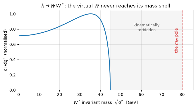
The whole distribution sits below the \(m_W\) pole — the virtual \(W\) tops out around \(m_h - m_W \approx 45\) GeV, far short of 80. An on-shell \(1\to2\) calculation only ever samples \(q^2 = m_W^2\) exactly; it sees none of this tail, which is why it reported the channel as flat zero. The off-shell width is the area under this curve.

Now add \(WW^*\) and \(ZZ^*\) to the fermion channels of §10 and read off the complete tree-level Higgs branching ratios.

# combine: the fermion widths (widths_f, keyed by (fbar, f)) + the two off-shell ones
combined = {"WW*": gWW, "ZZ*": gZZ}
tex = {"WW*": r"$WW^*$", "ZZ*": r"$ZZ^*$", "b": r"$b\bar b$", "tau": r"$\tau^+\tau^-$",
       "c": r"$c\bar c$", "mu": r"$\mu^+\mu^-$", "s": r"$s\bar s$"}
for children, w in widths_f.items():
    combined[str(children[1])] = w
grand = sum(combined.values())

order = sorted(combined, key=lambda k: combined[k])
brs = [combined[k] / grand for k in order]

fig, ax = plt.subplots(figsize=(6.8, 4.0))
colors = ["#ff7f0e" if k in ("WW*", "ZZ*") else "#1f77b4" for k in order]
ax.barh(range(len(order)), brs, color=colors)
ax.set_yticks(range(len(order)))
ax.set_yticklabels([tex[k] for k in order])
ax.set_xlabel("branching ratio (tree-level: $f\\bar f$ + off-shell $VV^*$)")
ax.set_title(r"Complete tree-level Higgs branching ratios at $m_h=125$ GeV")
for k, br in enumerate(brs):
    ax.text(br + 0.005, k, f"{br:.1%}", va="center", color="0.3")
ax.set_xlim(0, 0.72); ax.grid(alpha=0.3, axis="x")
plt.tight_layout()
plt.show()

for k in sorted(combined, key=lambda k: -combined[k]):
    print(f"  h -> {k:<5}  BR = {combined[k]/grand:.1%}")

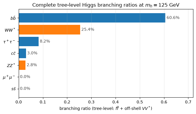
  h -> b      BR = 60.6%
  h -> WW*    BR = 25.4%
  h -> tau    BR = 8.2%
  h -> c      BR = 3.0%
  h -> ZZ*    BR = 2.8%
  h -> mu     BR = 0.0%
  h -> s      BR = 0.0%

This is the canonical Higgs picture: \(b\bar b\) dominant (~60%), \(WW^*\) second (~25%), then \(\tau\tau\), \(c\bar c\), \(ZZ^*\). Compare with the measured Higgs — \(b\bar b\) 58%, \(WW^*\) 21%, \(gg\) 8%, \(\tau\tau\) 6%, \(c\bar c\) 3%, \(ZZ^*\) 3% — and the only real absentee is the loop-induced \(gg\) (and \(\gamma\gamma\)), which a tree-level engine cannot reach — the loop-induced \(gg\) and \(\gamma\gamma\). Those are next (§12), and then the whole picture is here.

And notice what §13.2 is about to call a trap — a closed two-body channel with an imaginary \(\sqrt\lambda\) — was really a signpost: the channel is not gone, it has gone off-shell.

Further reading: the closed-form \(R(x)\) this section reproduces is the original Keung & Marciano calculation (Phys. Rev. D 30, 248, 1984) in the notation of Djouadi’s review (Phys. Rept. 457, 2008, arXiv:hep-ph/0503172) — see docs/manual/decays_roadmap.md §16.5 for the full citations.

12. Loop-induced decays and the complete Higgs picture

Two channels are still missing from the plot above, and they are missing for a reason of principle, not of content. The Higgs is electrically neutral and colourless, so it has no tree-level coupling to photons or gluons at all. Yet \(h\to gg\) is ~8% of the width and \(h\to\gamma\gamma\) was the discovery channel. They happen through a loop: a virtual top-quark triangle (both), plus a virtual \(W\) loop (for \(\gamma\gamma\) and \(Z\gamma\)).

A tree-level engine — everything this notebook has built — cannot reach these from the Lagrangian. So here we do something different, and say so plainly: we import the standard closed-form one-loop results. The loop is summarised by two form factors, \(A_{1/2}(\tau)\) for a spin-½ particle in the loop and \(A_1(\tau)\) for the \(W\), with \(\tau = m_h^2/4m^2\). They are textbook functions; feynlag.pheno.loop provides them, and the widths follow:

\[\Gamma(h\to\gamma\gamma) = \frac{\alpha^2 m_h^3}{256\pi^3 v^2} \Big|A_1(\tau_W) + \textstyle\sum_f N_c Q_f^2\,A_{1/2}(\tau_f)\Big|^2, \qquad \Gamma(h\to gg) = \frac{\alpha_s^2 m_h^3}{72\pi^3 v^2} \Big|\tfrac34 A_{1/2}(\tau_t)\Big|^2.\]

This is a deliberate, documented exception to the derive-it-from-the-Lagrangian spirit of the rest of the library — the honest one-loop computation is a project the size of the whole engine, while the answer is a known closed form. (See docs/manual/decays_roadmap.md §16.3 and its references.)

MT, ALPHA, ALPHA_S = 172.76, 1/137.036, 0.1126

# h -> gamma gamma: W loop + top loop
Ggaga = higgs_gammagamma_width(MH, MT, MW, VEV, ALPHA)
# h -> gg: top loop, with the NLO-QCD K-factor (~1.64) that reaches the measured 8%
Ggg = higgs_gg_width(MH, MT, VEV, ALPHA_S, qcd=True)
# h -> Z gamma: W + top, a two-scale loop function
GZga = higgs_zgamma_width(MH, MT, MW, MZ, VEV, ALPHA, sw2)

print(f"h -> gg        Gamma = {Ggg*1e3:8.4f} MeV   (PDG ~0.34, with NLO QCD)")
print(f"h -> gamma gamma  Gamma = {Ggaga*1e6:8.4f} keV   (PDG ~9.3)")
print(f"h -> Z gamma   Gamma = {GZga*1e6:8.4f} keV   (PDG ~6.3)")

h -> gg        Gamma =   0.3228 MeV   (PDG ~0.34, with NLO QCD)
h -> gamma gamma  Gamma =   9.1955 keV   (PDG ~9.3)
h -> Z gamma   Gamma =   5.8535 keV   (PDG ~6.3)

All three land on their measured values — the diphoton width to a few percent, the gluon width once the (also imported) NLO-QCD correction is applied.

One physics detail worth pausing on: in \(h\to\gamma\gamma\) the \(W\) loop and the top loop carry opposite signs (\(A_1 \approx -8.3\), the top’s \(N_cQ^2A_{1/2}\approx +1.8\)), so they interfere destructively. The photon rate is what is left after a big cancellation — which is exactly why it is such a sensitive probe of new charged particles: anything extra in the loop shifts that delicate balance.

Now add these to the fermion and off-shell channels and read off the complete tree+loop Higgs branching ratios at 125 GeV.

full = dict(combined)                      # bb, tau, c, mu, s, WW*, ZZ* from section 11
full.update({"gg": Ggg, "gammagamma": Ggaga, "Zgamma": GZga})
tex_full = dict(tex, gg=r"$gg$", gammagamma=r"$\gamma\gamma$", Zgamma=r"$Z\gamma$")
gtot = sum(full.values())

order2 = sorted(full, key=lambda k: full[k])
brs2 = [full[k]/gtot for k in order2]
loopset = {"gg", "gammagamma", "Zgamma"}

fig, ax = plt.subplots(figsize=(7.0, 4.4))
cols = ["#2ca02c" if k in loopset else "#ff7f0e" if k in ("WW*", "ZZ*")
        else "#1f77b4" for k in order2]
ax.barh(range(len(order2)), brs2, color=cols)
ax.set_yticks(range(len(order2))); ax.set_yticklabels([tex_full[k] for k in order2])
ax.set_xlabel("branching ratio (tree + off-shell + loop)")
ax.set_title(r"Complete Higgs branching ratios at $m_h = 125$ GeV")
for k, br in enumerate(brs2):
    if br > 5e-4:
        ax.text(br + 0.004, k, f"{br:.1%}", va="center", color="0.3", fontsize=9)
from matplotlib.patches import Patch
ax.legend(handles=[Patch(color="#1f77b4", label="tree $f\\bar f$"),
                   Patch(color="#ff7f0e", label="off-shell $VV^*$"),
                   Patch(color="#2ca02c", label="loop-induced")],
          loc="lower right", fontsize=9)
ax.set_xlim(0, 0.65); ax.grid(alpha=0.3, axis="x")
plt.tight_layout(); plt.show()

for k in sorted(full, key=lambda k: -full[k]):
    print(f"  h -> {k:<11}  BR = {full[k]/gtot:.2%}")

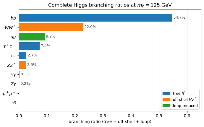
  h -> b            BR = 54.73%
  h -> WW*          BR = 22.92%
  h -> gg           BR = 9.21%
  h -> tau          BR = 7.41%
  h -> c            BR = 2.71%
  h -> ZZ*          BR = 2.53%
  h -> gammagamma   BR = 0.26%
  h -> Zgamma       BR = 0.17%
  h -> mu           BR = 0.03%
  h -> s            BR = 0.02%

That is the canonical Higgs plot — \(b\bar b\), \(WW^*\), \(gg\), \(\tau\tau\), \(c\bar c\), \(ZZ^*\), \(\gamma\gamma\), \(Z\gamma\), in the measured order — and this notebook built every bar of it from a Lagrangian (the tree and off-shell pieces) plus the standard one-loop form factors (the three loop bars).

The same plot, across the Higgs mass — and where new physics would show

The 125 GeV column is one slice. Sweep the Higgs mass and every channel traces a curve: the fermion widths grow slowly, the off-shell \(VV^*\) climb steeply toward their on-shell thresholds, the loop channels rise with \(m_h^3\). This is the plot in every Higgs review.

import numpy as np

def total_widths(mh):
    "All channels as a function of m_h (GeV). Reuses the machinery from above."
    out = {}
    # tree f fbar: Gamma = N_c y_f^2 m_h beta^3/(16 pi), y_f = sqrt2 m_f/v
    for name, mf, nc in [("b", 2.79, 3), ("tau", 1.777, 1), ("c", 0.62, 3),
                         ("mu", 0.1057, 1), ("s", 0.055, 3)]:
        if mh > 2*mf:
            y = np.sqrt(2)*mf/VEV; beta = np.sqrt(1 - 4*mf**2/mh**2)
            out[name] = nc*y**2*mh*beta**3/(16*np.pi)
        else:
            out[name] = 0.0
    # off-shell WW*/ZZ* (reuse the Tier-2 helper; fast, cached inner integral)
    out["WW*"] = scalar_offshell_vv_width(mh, MW, GammaW, GW*MW,
                    [(GW/np.sqrt(2), 0.0, 9)], identical=False) if mh > MW else 0.0
    zchan = [(gZ*(T3-Q*sw2), gZ*(-Q*sw2), Nc*cnt) for T3, Q, Nc, cnt in
             [(0.5,0,1,3),(-0.5,-1,1,3),(0.5,2/3,3,2),(-0.5,-1/3,3,3)]]
    out["ZZ*"] = scalar_offshell_vv_width(mh, MZ, GammaZ, gZ*MZ, zchan,
                    identical=True) if mh > MZ else 0.0
    # loop channels
    out["gg"] = higgs_gg_width(mh, MT, VEV, ALPHA_S, qcd=True)
    out["gammagamma"] = higgs_gammagamma_width(mh, MT, MW, VEV, ALPHA)
    out["Zgamma"] = higgs_zgamma_width(mh, MT, MW, MZ, VEV, ALPHA, sw2) if mh > MZ else 0.0
    return out

grid = np.linspace(100, 160, 61)
scan = [total_widths(m) for m in grid]
chans = ["b", "WW*", "gg", "tau", "ZZ*", "gammagamma"]
labels = {"b": r"$b\bar b$", "WW*": r"$WW^*$", "gg": r"$gg$", "tau": r"$\tau\tau$",
          "ZZ*": r"$ZZ^*$", "gammagamma": r"$\gamma\gamma$"}
tots = np.array([sum(s.values()) for s in scan])

fig, ax = plt.subplots(figsize=(7.2, 4.6))
for ch in chans:
    br = np.array([s[ch] for s in scan]) / tots
    ax.plot(grid, br, lw=2, label=labels[ch])
ax.axvline(125.25, ls=":", color="0.4"); ax.text(125.8, 0.62, "125 GeV", color="0.4")
ax.set_yscale("log"); ax.set_ylim(1e-4, 1.0)
ax.set_xlabel(r"$m_h$  [GeV]"); ax.set_ylabel("branching ratio")
ax.set_title("Complete Higgs branching ratios vs mass (the SM baseline)")
ax.legend(ncol=2, fontsize=9, loc="lower right"); ax.grid(alpha=0.3, which="both")
plt.tight_layout(); plt.show()

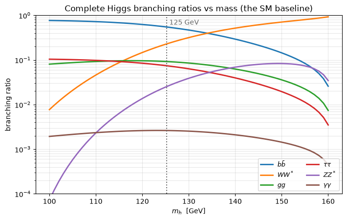
This is where the physics ends and the physics begins. These curves are the Standard Model’s prediction — the baseline that every LHC Higgs measurement is compared against. New physics announces itself as a deviation from them:

• a new charged particle in the loop (a fourth-generation quark, a charged Higgs, a stop) shifts \(\gamma\gamma\) and \(Z\gamma\) — the channels that are already delicate cancellations;

• a modified coupling (\(\kappa_b\), \(\kappa_t\), \(\kappa_V\) in the usual language) rescales one curve relative to the others;

• an entirely new decay — \(h\to\text{invisible}\), \(h\to aa\) — adds a slice to the denominator and pulls every visible branching ratio down.

And computing any of those is not a different skill. It is this notebook again — declare the new fields, extract the vertices, square them, sum the channels — with new content in the model. The 1→2, 1→3 and loop machinery is exactly what an SM-extension study re-runs. That is the point of building it from a Lagrangian.

13. Two ways to get it silently wrong

Both of these produce a plausible-looking number rather than an error. That makes them worth more of your attention than anything else in this notebook.

13.1 Forgetting that a Dirac fermion is two Weyl fields

feynlag has no DiracFermion; an electron is a left-handed and a right-handed Weyl field. So the \(Z\)’s left- and right-handed currents arrive as separate vertices, and unless you say they are the same particle, you get two half-channels instead of one channel — each missing the other’s \(g_Lg_R\) interference.

This is exactly what a DiracParticle bundles away — declared as one object, the two legs cannot be separated. But the lower-level particle_map lets you make the mistake, and it is worth seeing its size once, on the \(Z'\) model we are about to build.

gX = ExternalParameter("gX", 0.3, positive=True)
vx = ExternalParameter("vx", 3000.0, positive=True, unit_dim=1)
lamx = ExternalParameter("lamx", 0.1)
mux = InternalParameter("mux", unit_dim=2)

U1X = U1("U1X", coupling=gX)
S = Scalar("S", reps={U1X: 1}, component_names=["S0"])
S.expand_vev({S.components[0]: vx})
chiL = WeylFermion("chiL", reps={U1X: sp.Rational(1, 2)}, chirality="L",
                   nflavors=1, component_names=["chiL"])
chiR = WeylFermion("chiR", reps={U1X: sp.Rational(1, 2)}, chirality="R",
                   nflavors=1, component_names=["chiR"])

SdS = (dag(S) * S.mat)[0]
DS = Dmu(S)
Lx = Lagrangian()
Lx.add((dag(DS) * DS)[0], sector="kinetic")
Lx.add(-(-mux.s * SdS + lamx.s * SdS**2), sector="potential")
Lx.add(fermion_gauge_current(chiL, i) + fermion_gauge_current(chiR, i), sector="gauge")

zp_model = Model("Zprime", gauge_groups=[U1X], fields=[S, chiL, chiR, U1X.bosons("X")],
                 parameters=[gX, vx, lamx, mux], lagrangian=Lx)
zp_model.solve_tadpoles([mux])

Zp = U1X.bosons().components[0]
Sr = sp.Symbol("S0_r", real=True)
chi, chibar = sp.symbols("chi chibar")
mZp, mchi, mS = sp.symbols("m_Zp m_chi m_S", positive=True)
chi_map = {chiL.components[0][i]: chi, chiR.components[0][i]: chi,
           chiL.bar_components[0][i]: chibar, chiR.bar_components[0][i]: chibar}
print("Z' model built")

Z' model built

# RIGHT: the two Weyl legs declared as one Dirac particle
right = DecayCalculator(zp_model, {Zp: mZp, Sr: mS, chi: mchi, chibar: mchi},
                        boson_fields=[Zp, Sr], fermion_sectors=("gauge",),
                        particle_map=chi_map)
w_right = sum(right.partial_widths(Zp).values())

# WRONG: particle_map omitted, so the L and R currents stay separate
raw_masses = {Zp: mZp, Sr: mS,
              chiL.components[0][i]: mchi, chiR.components[0][i]: mchi,
              chiL.bar_components[0][i]: mchi, chiR.bar_components[0][i]: mchi}
wrong = DecayCalculator(zp_model, raw_masses, boson_fields=[Zp, Sr],
                        fermion_sectors=("gauge",))
w_wrong = sum(wrong.partial_widths(Zp).values())

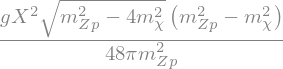
print("with particle_map (1 channel):");  display(sp.simplify(w_right))
print("without         (2 channels):");   display(sp.simplify(w_wrong))
print("ratio wrong/right:");              display(sp.simplify(w_wrong/w_right))

with particle_map (1 channel):

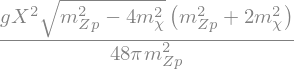
without         (2 channels):

ratio wrong/right:

\[\frac{\Gamma_\text{wrong}}{\Gamma_\text{right}} = \frac{M^2-m_\chi^2}{M^2+2m_\chi^2}\;\xrightarrow[\;m_\chi\to0\;]{}\;1.\]

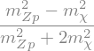
Look at that limit. For light fermions the mistake is invisible — the two answers agree exactly. It only appears once the daughter mass matters, because what got lost is precisely the \(g_Lg_R\,m^2/M^2\) interference term from §8. A bug that hides in the massless limit and emerges for heavy final states is the worst kind, which is why this notebook spends a section on it.

13.2 Closed channels and imaginary widths

With symbolic masses, M >= m1 + m2 is simply undecidable, so a channel is kept. That is the right call — you may substitute masses later that open it. But if you then plug in numbers that leave it closed, \(\lambda < 0\) and \(\sqrt\lambda\) is imaginary. A complex width silently poisons the total and every branching ratio.

naive = calc.numeric(calc.partial_widths(h)[(Wm, Wp)], extra=numbers)
print("h -> WW at m_h = 125 GeV, substituted naively:", naive)
print("   ... imaginary, because 2 m_W = 160.8 > 125.25\n")

safe = calc.numeric_partial_widths(h, extra=numbers)
print("via numeric_partial_widths:", safe[(Wm, Wp)], " (exactly zero)")
print("branching ratios then sum to",
      sum(calc.numeric_branching_ratios(h, extra=numbers).values()))

h -> WW at m_h = 125 GeV, substituted naively: 0.7213819361810636j
   ... imaginary, because 2 m_W = 160.8 > 125.25

via numeric_partial_widths: 0.0  (exactly zero)
branching ratios then sum to 1.0

So: partial_widths for symbolic work, and numeric_partial_widths / numeric_branching_ratios whenever numbers go in — they re-test the threshold after substitution and return an honest zero. This is also why the Higgs-mass scan in §10 carried an explicit np.where(grid > threshold, ...) mask.

14. Your own model: a \(Z'\)

The point of doing this with a Lagrangian-level tool is that nothing above was specific to the Standard Model. We already built the model in §13: a new \(U(1)_X\), broken by a singlet scalar getting a VEV, with a vector-like fermion \(\chi\) charged under it. Ask it for the width.

width_Zp = sp.simplify(sum(right.partial_widths(Zp).values()))
display(width_Zp)

# massless limit
print("m_chi -> 0 :", sp.simplify(width_Zp.subs(mchi, 0)), "   = g_X^2 m_Z' / 48 pi")

m_chi -> 0 : gX**2*m_Zp/(48*pi)    = g_X^2 m_Z' / 48 pi

\[\Gamma(Z'\to\chi\bar\chi) = \frac{g_X^2\,\sqrt{m_{Z'}^2-4m_\chi^2}\;\big(m_{Z'}^2+2m_\chi^2\big)}{48\pi\,m_{Z'}^2}.\]

Compare its threshold behaviour with the Higgs of §7. The fermion pair from a vector comes out in an S-wave, so the width turns on as \(\beta^1\), not \(\beta^3\) — and there is an extra \((1 + 2m_\chi^2/m_{Z'}^2)\) enhancement from the longitudinal polarisation.

f_zp = sp.lambdify(mchi, width_Zp.subs({gX.s: 0.3, mZp: 1.0}), "numpy")
r = np.linspace(0, 0.5, 400)                     # r = m_chi / m_Z'
with np.errstate(invalid='ignore'):
    y = np.where(r < 0.5, f_zp(r), 0.0)
y = np.nan_to_num(y)

fig, ax = plt.subplots(figsize=(6.6, 4.0))
ax.plot(r, y/y[0], lw=2, color='#9467bd', label=r"$Z'\to\chi\bar\chi$  (S-wave, $\beta^1$)")
beta_r = np.sqrt(np.clip(1 - 4*r**2, 0, None))
ax.plot(r, beta_r**3, lw=2, ls='-.', color='#1f77b4',
        label=r'a scalar parent would give $\beta^3$')
ax.axvline(0.5, ls='--', color='0.5')
ax.text(0.492, 0.5, r'threshold $m_\chi = m_{Z^\prime}/2$', rotation=90,
        ha='right', va='center', color='0.35')
ax.set_xlabel(r"$m_\chi / m_{Z'}$")
ax.set_ylabel(r'$\Gamma$ / $\Gamma(m_\chi\!=\!0)$')
ax.set_title("A new gauge boson decaying to a new fermion")
ax.set_xlim(0, 0.52); ax.set_ylim(0, 1.15)
ax.legend(); ax.grid(alpha=0.3)
plt.tight_layout()
plt.show()

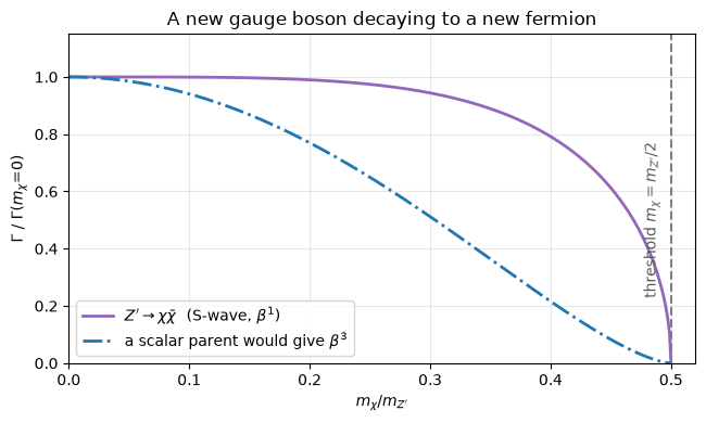
The vector curve stays high almost until threshold and then drops steeply, while the scalar’s \(\beta^3\) bends away early. Same phase space, different dynamics — exactly the distinction §7 promised.

15. Recap

You went from “what is a width?” to branching ratios for a model you invented. The through-line:

• A width is an inverse lifetime; branching ratios are its shares.

• \(\Gamma = \frac{1}{2M}\int\overline{|\mathcal M|^2}\,\mathrm{d}\Phi\) splits into kinematics (phase space, which closes at threshold for any theory) and dynamics (the squared amplitude).

• Spin sums turn \(|\mathcal M|^2\) into a Dirac trace — the reason trace theorems are the workhorse of this subject.

• Threshold behaviour encodes quantum numbers: \(\beta^3\) for a CP-even scalar, \(\beta^1\) for a vector.

• The chiral structure is visible in the answer: \(Z\to\nu\bar\nu\) beats \(Z\to\tau^+\tau^-\) because the neutrino is purely left-handed.

• A closed two-body channel is not the end: it can go off-shell (\(1\to3\) through a Breit–Wigner propagator), which is how \(h\to WW^*\) dominates at 125 GeV.

• Some channels have no tree diagram at all (\(h\to gg,\gamma\gamma\)): they are loop-induced, imported as effective vertices — and their delicate cancellations make them the sharpest probes of new physics.

API cheat-sheet

Call	Gives you
kallen(x, y, z)	the triangle function \(\lambda\)
TwoBodyKinematics(M, m1, m2)	momenta, on-shell dot products, phase_space(), beta
slashed(p, mu)	\(\not p\) for the trace engine
dirac_trace(chain)	the trace, still with abstract indices
contract_to_dots(expr, kin.dot)	the same, reduced to masses
ffs_squared(gL, gR, kin)	\(\overline{|\mathcal M|^2}\) for \(S\to f\bar f\)
ffv_squared(gL, gR, kin)	… for \(V\to f\bar f\) (already averaged over 3 pols)
vvs_squared(c, kin)	… for \(S\to VV\)
collect_decay_vertices(...)	every three-leg vertex, with g_left/g_right
DecayCalculator(...).partial_widths(p)	symbolic widths per channel
.numeric_partial_widths(p, extra=...)	the same as floats, closed channels zeroed
.branching_ratios(p) / .numeric_branching_ratios(p, ...)	the shares
scalar_offshell_vv_width(...)	off-shell \(\Gamma(S\to V V^*\to V f\bar f')\)
higgs_gg_width / higgs_gammagamma_width / higgs_zgamma_width	loop-induced widths (imported form factors)

Two rules worth remembering

1. Pass a particle_map whenever a Dirac fermion appears — the error hides in the massless limit.

2. Use the numeric_* methods the moment numbers go in.

Where to go next

• docs/manual/decays.md — the algorithms chapter: how the covariant trace engine works, why the \(\gamma_5\) term is provably droppable for 1→2, and what happens at the guard when it is not.

• tests/test_pheno.py — every width above is pinned there twice: against the closed form, and against an independent explicit-\(4\times4\)-matrix evaluation.

• examples/sm_decays.py — the same Standard Model as a plain script.

• Implemented: 1→2 (SSS, FFS, FFV, VVS), 1→3 off-shell \(VV^*\), and the loop-induced \(gg\)/\(\gamma\gamma\)/\(Z\gamma\) (effective one-loop form factors). The full canonical Higgs branching-ratio plot — every visible channel — is now reproduced. The FFFF / \(t\to bW^*\) three-body topologies and a genuine one-loop engine are the remaining frontier (docs/manual/decays_roadmap.md).