The type-I seesaw in `feynlag`: Majorana neutrino masses, step by step¶

Neutrinos are massless in the Standard Model. The type-I seesaw is the simplest way to give them mass: add right-handed neutrinos \(\nu_R\) (complete gauge singlets) with

a Dirac Yukawa \(-Y_\nu \bar L \tilde H\, \nu_R\) (like every other fermion), and
a Majorana mass \(-\tfrac12 M_R\, \nu_R^T C \nu_R\) — allowed precisely because \(\nu_R\) carries no gauge charge, and the origin of the mechanism.

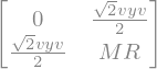
After electroweak symmetry breaking the neutral-fermion mass matrix, in the left-handed basis \(n = (\nu_L,\ \nu_R^c)\), is

\[\begin{split}M_\nu = \begin{pmatrix} 0 & m_D \\ m_D^T & M_R \end{pmatrix},\qquad m_D = Y_\nu v/\sqrt2.\end{split}\]

For \(M_R \gg m_D\) this seesaws: a naturally tiny light neutrino \(m_\nu \approx -m_D M_R^{-1} m_D^T\) and a heavy state \(\approx M_R\), mixed by \(V \approx m_D M_R^{-1}\). This notebook walks the whole construction in feynlag — including extracting the physical heavy-neutrino couplings, which requires the Majorana machinery (diracC, MajoranaBilinear) and a charge-conjugation-aware mass-basis rotation, because the physical neutrinos are Majorana fields mixing \(\nu_L\) with the charge-conjugate \(\nu_R^c\).

We use one generation for transparency; the machinery is generation-general.

1. Symmetries, parameters, fields¶

import sympy as sp
sp.init_printing()

from feynlag import (
    Bilinear, DiracGamma, Dmu, ExternalParameter, InternalParameter, Lagrangian,
    MajoranaBilinear, MajoranaRotation, Model, Rotation, SU2, Scalar, U1,
    WeylFermion, dag, diagonalize_takagi, diracC, diracPL, diracPR,
    extract_fermion_vertices, fermion_gauge_current, fermion_mass_matrix,
    majorana_mass_matrix, rotation_2x2, seesaw_light_mass, seesaw_mass_matrix,
    weinberg_rotation, charged_current_rotation,
)

gw = ExternalParameter("gw", 0.6535, positive=True)
g1 = ExternalParameter("g1", 0.3580, positive=True)
SU2L, U1Y = SU2("SU2L", coupling=gw), U1("U1Y", coupling=g1)
v = ExternalParameter("v", 246.0, positive=True, unit_dim=1)
lam = ExternalParameter("lam", 0.129)
mu2 = InternalParameter("mu2", unit_dim=2)
yv = ExternalParameter("yv", 0.01, positive=True)              # Dirac Yukawa
MR = ExternalParameter("MR", 1.0e3, positive=True, unit_dim=1)  # seesaw scale

The right-handed neutrino is a total singlet — reps={} — which is exactly what lets it carry a bare Majorana mass (nothing forbids \(\nu_R^T C \nu_R\)).

H = Scalar("H", reps={SU2L: 2, U1Y: sp.Rational(1, 2)}, component_names=["Gp", "H0"])
H.expand_vev({H.components[1]: v})
Ll = WeylFermion("Ll", reps={SU2L: 2, U1Y: -sp.Rational(1, 2)}, chirality="L",
                 nflavors=1, component_names=["nuL", "eL"])
eR = WeylFermion("eR", reps={U1Y: -1}, chirality="R", nflavors=1, component_names=["eR"])
nuR = WeylFermion("nuR", reps={}, chirality="R", nflavors=1, component_names=["nuR"])
print("ν_R reps (total singlet):", nuR.reps)

ν_R reps (total singlet): {}

2. The neutrino Lagrangian¶

The Dirac Yukawa uses the conjugate doublet \(\tilde H = (H^{0*},\,-H^{+*})\) (the same pattern as the up-type quarks). The Majorana mass is written with the MajoranaBilinear \(\nu_R^T C\,P_L\,\nu_R\) — feynlag’s charge-conjugation-aware sandwich (the middle carries diracC, the charge-conjugation matrix \(C=i\gamma^2\gamma^0\)).

i, j = sp.symbols("i j", integer=True)
Gp, H0 = H.components
nuL, eL = Ll.components
nuLbar, eLbar = Ll.bar_components
nR, nRbar = nuR.components[0], nuR.bar_components[0]
CPL = diracC * diracPL

# Dirac Yukawa via H̃:  −Y_ν L̄ H̃ ν_R + h.c.
LYukD = -(yv.s * sp.conjugate(H0) * Bilinear(nuLbar[i], diracPR, nR[j])
          + yv.s * (-sp.conjugate(Gp)) * Bilinear(eLbar[i], diracPR, nR[j]))
LYukD += -(sp.conjugate(yv.s) * H0 * Bilinear(nRbar[j], diracPL, nuL[i])
           + sp.conjugate(yv.s) * (-Gp) * Bilinear(nRbar[j], diracPL, eL[i]))

# Right-handed Majorana mass:  −½ M_R ν_Rᵀ C ν_R + h.c.
op = -sp.Rational(1, 2) * MR.s * MajoranaBilinear(nR[i], CPL, nR[j])
LMaj = op + sp.conjugate(op)

current = fermion_gauge_current(Ll, i) + fermion_gauge_current(eR, i)
display(MajoranaBilinear(nR[i], CPL, nR[j]))

../_images/80b43e24c9cb53225e2888ed0fe72424f901c9c3b222b6cadeb9629f7880459e.png

3. Assemble the model and check invariance¶

L = Lagrangian()
L.add((dag(Dmu(H)) * Dmu(H))[0], sector="kinetic")
L.add(-(-mu2.s * (dag(H) * H.mat)[0] + lam.s * (dag(H) * H.mat)[0]**2), sector="potential")
L.add(LYukD + current, sector="yukawa")
L.add(LMaj, sector="other")      # the Majorana mass — a mass term, not a vertex

model = Model("SM-seesaw", gauge_groups=[SU2L, U1Y],
              fields=[H, Ll, eR, nuR, SU2L.bosons("W"), U1Y.bosons("B")],
              parameters=[gw, g1, v, lam, mu2, yv, MR], lagrangian=L)
print(model.check_invariance())
model.check_invariance().raise_on_failure()
print("tadpole:", model.solve_tadpoles([mu2]))

InvarianceReport(16 checks, OK)

tadpole: {mu2: lam*v**2}

Gauge invariance passes: the Dirac Yukawa is a standard singlet-completing coupling, and the Majorana mass is invariant because \(\nu_R\) is a total singlet. Now rotate the gauge bosons to the mass basis (Weinberg + \(W^\pm\)), as usual.

# physical basis: the standard Weinberg + W± rotations, from feynlag.models
Z, A = weinberg_rotation(model, SU2L, U1Y)
Wp, Wm = charged_current_rotation(model, SU2L)

4. The seesaw mass matrix¶

The Dirac block comes from the Yukawa (fermion_mass_matrix), the Majorana block from majorana_mass_matrix (the symmetric \(M_R\) — the D.2 Majorana machinery), and seesaw_mass_matrix assembles the symmetric \(6N\times6N\) block form.

mD = fermion_mass_matrix(LYukD, nuLbar, nR, model.vacuum, 1, (i, j), gamma=diracPR)
MRmat = majorana_mass_matrix(LMaj, nR, model.vacuum, 1, (i, j), gamma=CPL)
Mnu = seesaw_mass_matrix(mD, MRmat)
print("Dirac mass m_D = Y_ν v/√2:", mD[0, 0], "   Majorana mass M_R:", MRmat[0, 0])
Mnu

Dirac mass m_D = Y_ν v/√2: sqrt(2)*v*yv/2    Majorana mass M_R: MR

../_images/995485578aca14eb771824b1a78b2be64deb1daf73ba73e5d2263f89e5fadf97.png

5. The seesaw formula and the spectrum¶

Block-diagonalising for \(M_R \gg m_D\) gives the light neutrino mass \(m_\nu \approx -m_D M_R^{-1} m_D^T = -m_D^2/M_R\) — the seesaw: heavy \(M_R\) in the denominator makes \(m_\nu\) tiny. We check it against the exact Takagi factorisation of the full matrix.

print("seesaw formula  m_ν = −m_D²/M_R  =", sp.simplify(seesaw_light_mass(mD, MRmat)[0, 0]))

bench = {yv.s: 0.01, v.s: 246.0, MR.s: 1000.0, gw.s: 0.6535, g1.s: 0.3580}
Mn = sp.Matrix(2, 2, lambda a, b: sp.nsimplify(Mnu[a, b].subs(bench)))
U, D = diagonalize_takagi(Mn)     # M = U D Uᵀ, D ≥ 0 (Takagi, for Majorana)
masses = [abs(complex(sp.N(D[k, k]))) for k in range(2)]
light = 0 if masses[0] < masses[1] else 1
heavy = 1 - light
print(f"exact spectrum:  m_light = {masses[light]:.4e} GeV,  m_heavy = {masses[heavy]:.1f} GeV")
print(f"seesaw formula:  m_light = {abs(complex(sp.N(seesaw_light_mass(mD, MRmat)[0,0].subs(bench)))):.4e} GeV")

seesaw formula  m_ν = −m_D²/M_R  = -v**2*yv**2/(2*MR)

exact spectrum:  m_light = 3.0258e-03 GeV,  m_heavy = 1000.0 GeV
seesaw formula:  m_light = 3.0258e-03 GeV

The exact light mass and the seesaw formula agree. The spectrum is one light state and one heavy state \(\approx M_R\).

The seesaw tension. Here \(M_R = 1\) TeV gives \(m_\nu \approx 3\) MeV — far too heavy. A realistic \(m_\nu \sim 0.05\) eV needs \(M_R \sim 10^{14}\) GeV (with \(Y_\nu \sim 1\)), which pushes the heavy neutrino — and its couplings — out of experimental reach. We keep \(M_R = 1\) TeV here so the mixing below is visible.

6. The light–heavy mixing¶

The physical neutrinos are Majorana mass eigenstates \(\chi_k\) mixing \(\nu_L\) with \(\nu_R^c\). The light–heavy mixing \(V\) — the \(\nu_L\) content of the heavy state — is the \((0,\text{heavy})\) entry of \(U^*\), and equals \(\approx m_D/M_R\). It controls every heavy-neutrino coupling.

V = abs(complex(sp.N(U.conjugate()[0, heavy])))
print(f"light–heavy mixing V = |U*[0,heavy]| = {V:.5f}")
print(f"           m_D/M_R               = {float((mD[0,0]/MR.s).subs(bench)):.5f}")

light–heavy mixing V = |U*[0,heavy]| = 0.00174
           m_D/M_R               = 0.00174

7. Rotate to the physical Majorana basis¶

MajoranaRotation substitutes the weak neutrinos into the physical Majorana fields \(\chi_k\) using the Takagi \(U\). Because \(\chi\) is self-conjugate (\(\chi^c=\chi\)), the four Weyl fields map as

\[\nu_L\to U^*\,P_L\chi,\quad \bar\nu_L\to U\,\bar\chi P_R,\quad \nu_R\to U\,P_R\chi,\quad \bar\nu_R\to U^*\,\bar\chi P_L,\]

which is exactly the charge-conjugation bookkeeping feynlag’s Rotation cannot express (it is square and conjugation-blind). We apply it to the current sector and extract the physical vertices.

chiL, chiR = sp.IndexedBase("chiL"), sp.IndexedBase("chiR")
chiLbar, chiRbar = sp.IndexedBase("chiLbar"), sp.IndexedBase("chiRbar")
rot = MajoranaRotation(U, nuL, nR, nuLbar, nRbar, chiL, chiR, chiLbar, chiRbar, n_L=1)
Lchi = rot.apply(model.physical_lagrangian(sector="yukawa"), (i, j), 1)
tab = extract_fermion_vertices(Lchi, [Wp, Wm, Z])
print("extracted", len(tab), "neutrino vertex groups in the physical basis")

extracted 22 neutrino vertex groups in the physical basis

8. The heavy-neutrino couplings¶

The smoking gun: the charged-current production coupling \(W\,\bar\ell\,N = (g/\sqrt2)\,V\) — the heavy neutrino couples to \(W\) only through the mixing \(V\). The light neutrino keeps the full SM coupling.

mu = sp.Symbol("mu", integer=True)
gL = DiracGamma(mu) * diracPL
gsq = float((gw.s / sp.sqrt(2)).subs(bench))
gz = float(sp.sqrt(gw.s**2 + g1.s**2).subs(bench))

def coup(key, boson, norm):
    c = tab.get(key, {}).get(1, {}).get((boson,), 0)
    return abs(complex(sp.N(sp.simplify(c).subs(bench)))) / norm if c != 0 else 0.0

for k, name in ((light, "light ν"), (heavy, "heavy N")):
    cW = coup((eLbar[0], gL, chiL[k]), Wm, gsq)
    print(f"  W⁻ e {name}:  |coupling|/(g/√2) = {cW:.5f}")
for k, name in ((light, "light ν"), (heavy, "heavy N")):
    cZ = coup((chiLbar[light], gL, chiL[k]), Z, gz)
    print(f"  Z ν {name}:   |coupling|/g_Z    = {cZ:.5f}")

  W⁻ e light ν:  |coupling|/(g/√2) = 1.00000
  W⁻ e heavy N:  |coupling|/(g/√2) = 0.00174

  Z ν light ν:   |coupling|/g_Z    = 0.50000
  Z ν heavy N:   |coupling|/g_Z    = 0.00087

The heavy-neutrino couplings are suppressed by the mixing \(V\approx m_D/M_R\): \(W\bar eN = (g/\sqrt2)\,V\), \(Z\bar\nu N = (g_Z/2)\,V\) (up to the neutral-current \(\tfrac12\)). The light neutrino keeps the SM values \(g/\sqrt2\) and \(g_Z/2\).

9. Decoupling¶

Raising \(M_R\) drives the mixing — and the heavy-neutrino production coupling — to zero as \(1/M_R\): the seesaw decouples. This is the same computation at three scales.

for MRval in (1.0e3, 1.0e4, 1.0e5):
    b = dict(bench); b[MR.s] = MRval
    Mnk = sp.Matrix(2, 2, lambda a, bb: sp.nsimplify(Mnu[a, bb].subs(b)))
    Uk, Dk = diagonalize_takagi(Mnk)
    mk = [abs(complex(sp.N(Dk[c, c]))) for c in range(2)]
    hv = 0 if mk[0] > mk[1] else 1
    rk = MajoranaRotation(Uk, nuL, nR, nuLbar, nRbar, chiL, chiR, chiLbar, chiRbar, n_L=1)
    tk = extract_fermion_vertices(rk.apply(model.physical_lagrangian(sector="yukawa"), (i, j), 1), [Wp, Wm, Z])
    cW = tk.get((eLbar[0], gL, chiL[hv]), {}).get(1, {}).get((Wm,), 0)
    val = abs(complex(sp.N(sp.simplify(cW).subs(b)))) / gsq if cW != 0 else 0.0
    print(f"  M_R = {MRval:.0e} GeV:  m_light = {min(mk):.3e} GeV,  W e N /(g/√2) = {val:.3e}")

  M_R = 1e+03 GeV:  m_light = 3.026e-03 GeV,  W e N /(g/√2) = 1.739e-03

  M_R = 1e+04 GeV:  m_light = 3.026e-04 GeV,  W e N /(g/√2) = 1.739e-04

  M_R = 1e+05 GeV:  m_light = 3.026e-05 GeV,  W e N /(g/√2) = 1.739e-05

10. Recap¶

Starting from the SM plus right-handed neutrinos, feynlag delivered the type-I seesaw end to end:

Step	Tool	Result
Majorana mass	`MajoranaBilinear`, `majorana_mass_matrix`	the symmetric \(M_R\) block
Mass matrix	`seesaw_mass_matrix`, `diagonalize_takagi`	light + heavy spectrum
Seesaw formula	`seesaw_light_mass`	\(m_\nu = -m_D^2/M_R\), matching the exact Takagi
Physical basis	`MajoranaRotation`	\(\nu_L,\nu_R \to\) Majorana \(\chi\) (with \(\nu_R^c\))
Couplings	`extract_fermion_vertices`	\(W\bar\ell N=(g/\sqrt2)V\), decoupling as \(M_R\to\infty\)

The heavy neutrino’s couplings are fixed by a single number, the light–heavy mixing \(V \approx m_D/M_R\) — which is also what makes a high-scale seesaw experimentally invisible.

Where to go next: SM_Feynman_Rules_Tutorial for the full SM pipeline, SM_U1X_Tutorial for a \(Z'\), and ModelBuilding_Tutorial for the suggest/anomalies model-building tools.

The type-I seesaw in feynlag: Majorana neutrino masses, step by step¶