From Pauli matrices to any SU(N): gauge representations with feynlag

A gentle tour for someone new to particle physics — you need only linear algebra and a little quantum mechanics.

Quarks come in three colours. The weak force acts on doublets. Grand unified theories pack a whole matter generation into a \(\bar 5\) and a \(10\) of SU(5). Every one of these statements is about a representation of a Lie group — the mathematical language of gauge symmetry.

This notebook builds that language from the ground up, and shows how feynlag now constructs the generators of any SU(\(N\)) representation dynamically — with no hard-coded matrices beyond the familiar Pauli and Gell-Mann ones.

Roadmap

1. Symmetries and generators

2. The Lie algebra

3. Representations: one symmetry, many sizes

4. Labelling representations: dimension and Dynkin labels

5. A peek inside: highest weights and ladder operators

6. Conjugate representations: matter vs antimatter

7. Anomalies: a consistency test the representations must pass

8. Putting it to work: a model in a brand-new representation

9. Recap

import sympy as sp
sp.init_printing()   # pretty-print matrices as LaTeX

from feynlag import (SU2, SU3, SUN, Scalar, WeylFermion, Model,
                     ExternalParameter, Lagrangian, Dmu,
                     structure_constants, check_anomaly_free)
from feynlag.groups import sun

1. Symmetries and generators

A symmetry in particle physics acts on a multiplet of fields — a column of \(n\) objects that the transformation mixes among themselves. Mixing \(n\) things linearly is just multiplication by an \(n\times n\) matrix \(U\).

For a continuous symmetry we can turn the transformation on gently. Very close to “doing nothing” (\(U = \mathbb{1}\)), any such transformation looks like

\[U(\alpha) \;\approx\; \mathbb{1} + i\,\alpha\, T + \dots\]

The matrix \(T\) that appears at first order is a generator: it generates the whole family of transformations. A group with several independent “directions” of transformation has several generators \(T^a\) (\(a = 1, 2, \dots\)).

The smallest non-trivial example is SU(2), acting on a 2-component doublet (think of the weak isospin of \((\nu_e, e)_L\)). Its three generators in this 2-dimensional (fundamental) representation are the Pauli matrices divided by two:

SU2L = SU2('SU2L')
T = SU2L.generators(2)      # '2' = the 2-dimensional (fundamental) rep
T[0], T[1], T[2]

Two facts you can read straight off these matrices, both required of any generator of a special-unitary group:

• they are Hermitian (\(T = T^\dagger\)) — so that \(U = e^{i\alpha T}\) is unitary (probability-preserving),

• they are traceless — the “S” (for special) in SU(\(N\)).

all(Ta == Ta.conjugate().T for Ta in T), [sp.trace(Ta) for Ta in T]

(True, [0, 0, 0])

2. The Lie algebra: how generators multiply

Generators do not commute — that is what makes the group non-abelian and the physics rich. The way they fail to commute is the single most important piece of data about the group:

\[[T^a, T^b] \;=\; T^aT^b - T^bT^a \;=\; i\, f^{abc}\, T^c .\]

The numbers \(f^{abc}\) are the structure constants. They are the group, in the sense that everything else can be reconstructed from them.

Let us verify the relation for SU(2). Taking \(a=1, b=2\) (Python indices 0, 1), the commutator should come out equal to \(i\,T^3\):

comm = T[0] * T[1] - T[1] * T[0]
comm

sp.simplify(comm - sp.I * T[2])     # zero matrix  =>  f^{123} = +1

For SU(2) the structure constants are just the Levi-Civita symbol, \(f^{abc} = \varepsilon^{abc}\). feynlag can hand them to us as a dictionary of the non-zero entries:

structure_constants(SU2L)

One more standard convention: the generators are normalised so that

\[\mathrm{Tr}(T^a T^b) = \tfrac{1}{2}\,\delta^{ab}.\]

The matrix of all traces is therefore \(\tfrac12\) times the identity:

sp.Matrix(3, 3, lambda a, b: sp.trace(T[a] * T[b]))

3. Representations: one symmetry, many sizes

Here is the key idea. The same abstract symmetry can act on multiplets of different sizes — on a doublet, a triplet, an octet, …. Each such realisation is a representation: a set of matrices \(T^a\) (of some common size) obeying the same Lie algebra, i.e. with the same structure constants \(f^{abc}\).

Three representations exist for every group and deserve names:

• the singlet — a 1-dimensional field that does not transform at all (\(T^a = 0\)); it is neutral under the force.

• the fundamental — the smallest faithful one (\(N\times N\) for SU(\(N\))); quarks live in the fundamental 3 of colour SU(3).

• the adjoint — same dimension as the number of generators; it is built directly out of the structure constants, \((T^a)_{bc} = -i f^{abc}\). The force-carrying gauge bosons (gluons!) live here.

Let us look at colour SU(3). Its fundamental has eight \(3\times 3\) generators — the Gell-Mann matrices over two:

SU3c = SU3('SU3c')
lam = SU3c.generators(3)    # 8 generators, each 3x3
lam[0], lam[2], lam[7]

The adjoint (the 8, home of the gluons) is eight \(8\times 8\) matrices; the singlet is trivial. Same group, three different sizes:

print('fundamental 3:', lam[0].shape,
      '  adjoint 8:', SU3c.generators(8)[0].shape,
      '  singlet 1:', SU3c.generators(1)[0].shape)

fundamental 3: (3, 3)   adjoint 8: (8, 8)   singlet 1: (1, 1)

And — this is the whole point of the word representation — the octet obeys the same algebra as the triplet, with the very same \(f^{abc}\):

f3 = structure_constants(SU3c)
adj = SU3c.generators(8)
comm = adj[0] * adj[1] - adj[1] * adj[0]
rhs = sum((sp.I * f3.get((0, 1, c), 0) * adj[c] for c in range(8)), sp.zeros(8, 8))
sp.simplify(comm - rhs) == sp.zeros(8, 8)

True

4. Labelling representations: dimension and Dynkin labels

So far we used dimension labels: 1 (singlet), 3 (fundamental of SU(3)), 8 (adjoint). That is convenient but incomplete — for a general group there can be several representations of the same dimension, so dimension alone is ambiguous.

feynlag therefore lets you build any SU(\(N\)) with SUN(N, name), and label a representation in three ways:

• by its integer dimension (1, N, N\(^2-1\), or any dimension that is unambiguous),

• by an explicit Dynkin label — a tuple \((a_1, \dots, a_{N-1})\) of non-negative integers that names exactly one representation,

• by a conjugate label (Section 6).

Here is SU(4), with its singlet, fundamental (4) and adjoint (15):

SU4 = SUN(4, 'SU4')
[SU4.rep_dim(1), SU4.rep_dim(4), SU4.rep_dim(15)]

The dimension of any representation follows from its Dynkin labels through the Weyl dimension formula (a piece of pure combinatorics — no matrices are built to evaluate it). Here is a small catalogue of SU(3) representations, each named by its Dynkin label:

for dyn in [(0, 0), (1, 0), (0, 1), (1, 1), (2, 0), (0, 2), (3, 0)]:
    print(f'Dynkin {dyn}  ->  dimension {sun.weyl_dim(3, dyn)}')

Dynkin (0, 0)  ->  dimension 1
Dynkin (1, 0)  ->  dimension 3
Dynkin (0, 1)  ->  dimension 3
Dynkin (1, 1)  ->  dimension 8
Dynkin (2, 0)  ->  dimension 6
Dynkin (0, 2)  ->  dimension 6
Dynkin (3, 0)  ->  dimension 10

Notice that \((1,0)\) and \((0,1)\) are both 3-dimensional: they are the quark and antiquark representations (Section 6). Notice too that dimension \(15\) would be ambiguous. The resolver resolve_rep translates a friendly label into a canonical Dynkin tuple (plus a flag for whether it is conjugated), and it refuses to guess when a dimension is ambiguous:

sun.resolve_rep(3, 6), sun.resolve_rep(3, '3bar'), sun.resolve_rep(3, (2, 0))

(((2, 0), False), ((1, 0), True), ((2, 0), False))

try:
    sun.resolve_rep(3, 15)          # dimension 15 is ambiguous in SU(3)
except ValueError as e:
    print('ValueError:', e)

ValueError: SU(3) dimension 15 is ambiguous ((4, 0), (2, 1)); pass an explicit Dynkin tuple

5. A peek inside: highest weights and ladder operators

Where do the matrices for, say, the 6 of SU(3) actually come from? The construction is a direct generalisation of something you already know from quantum mechanics: building an angular-momentum multiplet with raising and lowering operators.

Recall the spin-\(j\) story. You start from the highest-weight state \(|j, j\rangle\) and apply the lowering operator \(J_-\) again and again to sweep out the whole multiplet \(|j, j-1\rangle, |j, j-2\rangle, \dots\). The matrix elements are square roots,

\[J_\pm\,|j, m\rangle = \sqrt{(j \mp m)(j \pm m + 1)}\;|j, m\pm 1\rangle .\]

A general SU(\(N\)) irrep is built exactly this way — pick the highest-weight state, then lower with the group’s ladder operators to fill in every state. (The systematic bookkeeping is the Gelfand–Tsetlin construction; feynlag does it for you.) The fingerprint is the same: the ladder matrix elements come out as square roots of rationals.

Watch it appear. Here is the 6 of SU(3) — six \(6\times 6\) generators — and its raising combination \(T^1 + iT^2\):

six = sun.su_n_generators(3, (2, 0))   # the 6 of SU(3)
raiser = six[0] + sp.I * six[1]
raiser

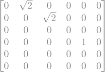
There are the tell-tale \(\sqrt{2}\)’s — the very same ladder structure as \(J_+\) in the spin story, now inside a colour representation.

And the pay-off that makes this a genuine representation: these six \(6\times 6\) matrices, produced purely by the ladder algorithm, satisfy the same structure constants \(f^{abc}\) as the \(3\times 3\) fundamental. The library shares one common basis across every representation precisely so this holds automatically:

def closes(T, f, dim, n=8):
    return all(
        sp.expand((T[a] * T[b] - T[b] * T[a])
                  - sum((sp.I * f.get((a, b, c), 0) * T[c] for c in range(n)),
                        sp.zeros(dim, dim))) == sp.zeros(dim, dim)
        for a in range(n) for b in range(n))

closes(six, f3, 6)     # the 6 obeys the SAME algebra as the 3

True

Finally, a representation carries an intrinsic number, its quadratic Casimir \(C_2 = \sum_a T^aT^a\), which is a multiple of the identity (a fact guaranteed by Schur’s lemma). For the 6 of SU(3) it is \(10/3\):

C2 = sum((Ta * Ta for Ta in six), sp.zeros(6, 6))
C2[0, 0], C2 == C2[0, 0] * sp.eye(6)

(10/3, True)

6. Conjugate representations: matter vs antimatter

For every representation \(R\) there is a conjugate representation \(\bar R\) — physically, the one the antiparticles live in. If quarks are a 3 of colour, antiquarks are a \(\bar{\mathbf 3}\). The generators of the conjugate are

\[\bar T^{\,a} = -\,(T^a)^{*} .\]

In feynlag you ask for a conjugate with a string like '3bar', a negative integer, or the reversed Dynkin tuple. It really is \(-(T^a)^*\):

three = SU3c.generators(3)
threebar = SU3c.generators('3bar')
all(tb == -t.conjugate() for tb, t in zip(threebar, three))

True

We already saw that the Dynkin label of \(\bar{\mathbf 3}\) is \((0,1)\), the reverse of the fundamental’s \((1,0)\):

sun.resolve_rep(3, '3bar')      # -> ((1, 0), True):  the conjugate of (1, 0)

((1, 0), True)

This is exactly why a quark (\(\mathbf 3\)) and an antiquark (\(\bar{\mathbf 3}\)) can bind into a colour-neutral singlet — a meson. Combining a representation with its conjugate always contains the singlet. (For a real representation, such as the SU(3) octet, \(R = \bar R\) and the distinction disappears.)

7. Anomalies: a consistency test the representations must pass

Not every collection of representations gives a healthy theory. In a chiral gauge theory (one where left- and right-handed fermions transform differently — like the real world), a quantum effect called the triangle anomaly can spoil the gauge symmetry unless it cancels between the particles. This is a genuine constraint that rules models in or out.

Each representation contributes an anomaly coefficient \(A(R)\), fixed by a symmetric trace of three generators and normalised to \(A(\text{fundamental}) = 1\). Here it is, written out transparently:

def anomaly_index(group, rep):
    T = group.generators(rep)
    TF = group.generators(group.N)           # the fundamental, for normalisation
    n = len(TF)
    for a in range(n):
        for b in range(a, n):
            for c in range(b, n):
                tF = sp.nsimplify(sp.expand(
                    sp.trace(TF[a] * (TF[b] * TF[c] + TF[c] * TF[b]))))
                if tF != 0:
                    num = sp.nsimplify(sp.expand(
                        sp.trace(T[a] * (T[b] * T[c] + T[c] * T[b]))))
                    return sp.simplify(num / tF)
    return sp.S.Zero

{'A(3)': anomaly_index(SU3c, 3), 'A(3bar)': anomaly_index(SU3c, '3bar'),
 'A(6)': anomaly_index(SU3c, 6), 'A(8)': anomaly_index(SU3c, 8)}

{'A(3)': 1, 'A(3bar)': -1, 'A(6)': 7, 'A(8)': 0}

A real (\(R=\bar R\)) representation like the 8 has \(A = 0\); a conjugate flips the sign, \(A(\bar R) = -A(R)\).

Now the famous example. In the SU(5) grand unified theory, one whole generation of matter fits into a left-handed \(\bar{\mathbf 5}\) plus a \(\mathbf{10}\). Individually each is anomalous — but their anomalies cancel, \(A(\bar{\mathbf 5}) + A(\mathbf{10}) = -1 + 1 = 0\). That near-miraculous cancellation is one of the reasons SU(5) was taken seriously as a unifying group:

SU5 = SUN(5, 'SU5')
anomaly_index(SU5, '5bar'), anomaly_index(SU5, (0, 1, 0, 0))   # 10 = (0,1,0,0)

And we can let the library confirm the cancellation on a real model — two left-handed fermion multiplets making up one generation, checked by check_anomaly_free. Note the fields are declared directly in the higher representations, including the \(\mathbf{10}\) by its Dynkin tuple:

five_bar = WeylFermion('fbar', reps={SU5: '5bar'}, chirality='L',
                       nflavors=1, component_names=[f'fb_{i}' for i in range(5)])
ten = WeylFermion('ften', reps={SU5: (0, 1, 0, 0)}, chirality='L',
                  nflavors=1, component_names=[f'ft_{i}' for i in range(10)])
generation = Model('SU5generation', gauge_groups=[SU5], fields=[five_bar, ten])
check_anomaly_free(generation).ok

True

8. Putting it to work: a model in a brand-new representation

None of this would matter if you could not use the new representations to build a Lagrangian. You can. Let us give a scalar field the fundamental of SU(4) — a group feynlag never had built in — and form its covariant derivative \(D_\mu S = \partial_\mu S - i g\,A^a_\mu T^a S\). The covariant derivative automatically uses the SU(4) fundamental generators we met above:

g4 = ExternalParameter('g4', 0.9, positive=True)
SU4c = SUN(4, 'SU4c', coupling=g4)
S = Scalar('S', reps={SU4c: 4}, component_names=[f'S_{i}' for i in range(4)])
DS = Dmu(S)
DS[0]      # first component of the covariant derivative

Finally, the acid test of a gauge theory: the Lagrangian must be gauge invariant. feynlag checks this end-to-end. Here we confirm that the mass term \(S^\dagger S\) is invariant under the full SU(4) — the machinery transforms the field with the GT-built generators and verifies the variation vanishes:

L = Lagrangian().add((S.dag() * S.mat)[0], sector='potential')
model = Model('SU4-scalar', gauge_groups=[SU4c], fields=[S],
              parameters=[g4], lagrangian=L)
model.check_invariance().ok

True

9. Recap

You have gone from “what is a generator?” to building a gauge-invariant term in an SU(4) theory. The through-line:

• A generator is the first-order piece of a continuous symmetry; the Lie algebra \([T^a,T^b]=if^{abc}T^c\) packages how they combine.

• A representation realises that algebra at a chosen size; every one shares the same structure constants \(f^{abc}\).

• feynlag builds the generators of any SU(\(N\)) representation on demand, by the highest-weight / ladder construction — no hard-coded matrices beyond Pauli and Gell-Mann.

Labelling cheat-sheet for SUN(N, name).generators(label):

Label	Meaning
1	singlet (trivial)
N	fundamental
N**2 - 1	adjoint
other int d	the unique dimension-d rep (error if ambiguous)
-d or 'dbar'	the conjugate of dimension d
Dynkin tuple (a_1, ..., a_{N-1})	that exact irrep (fully general)

To go deeper: tests/test_sun.py pins all of this physics (the SU(4)/SU(5) algebra, the 6 of SU(3), conjugates, the SU(5) \(\bar 5 + 10\) anomaly cancellation), and the groups/sun.py module docstring explains the Gelfand–Tsetlin construction and why the normalisation is fixed by the shared basis.