Feynman rules of the Standard Model with feynlag

This notebook walks through feynlag’s pipeline stage by stage: declare symmetries and fields, write the Lagrangian, check it, break the symmetry, diagonalize, and extract Feynman rules — using the electroweak sector of the Standard Model as the worked example. It ends with a guide to extending the model to a BSM scenario.

Every cell below is executed live against the actual library — nothing here is hand-typed output. All conventions (metric signature, P_L, the sign of D_μ, the explicit 1/√2 in VEVs, vertex normalization) are fixed once in CONVENTIONS.md; that file is the source of truth if a sign looks unfamiliar.

What we’re building: an SU(2)_L × U(1)_Y Higgs doublet with its potential and covariant kinetic term — enough to extract the Higgs self-couplings, gauge-boson masses, the Weinberg rotation, and every hVV/hhVV/Goldstone vertex.

import sympy as sp
from feynlag import (
    Bilinear, DiracGamma, Dmu, ExternalParameter, InternalParameter,
    Lagrangian, Model, Rotation, SU2, Scalar, U1, WeylFermion,
    conjugate_pair, cubic_couplings, dag, diracPL, diracPR,
    extract_fermion_vertices, fermion_feynman_rule, fermion_gauge_current,
    fermion_mass_matrix, latex_feynman_table, quartic_couplings,
    rotation_2x2,
)

sp.init_printing()

1. Declare the symmetries and parameters

• SU2/U1 are GaugeGroups carrying explicit generator matrices (σᵃ/2 for SU(2)); they build their own gauge-boson fields on demand.

• ExternalParameter is a number you feed in from experiment — it needs a value for benchmarking and later UFO export.

• InternalParameter is a symbol whose defining expression is derived later (here, by the tadpole condition in §6). unit_dim is the mass dimension, used by the dimension-≤-4 invariance check.

• positive=True lets SymPy simplify sqrt expressions involving v, gw, g1 without spurious branch-cut assumptions (the “positive dummy symbols” rule in CONVENTIONS.md).

gw = ExternalParameter("gw", 0.6535, positive=True)
g1 = ExternalParameter("g1", 0.3580, positive=True)
SU2L, U1Y = SU2("SU2L", coupling=gw), U1("U1Y", coupling=g1)

v   = ExternalParameter("v", 246.0, positive=True, unit_dim=1)
lam = ExternalParameter("lam", 0.129)
mu2 = InternalParameter("mu2", unit_dim=2)   # will be *derived*, not set

gw, g1, v, lam, mu2

(ExternalParameter('gw'),
 ExternalParameter('g1'),
 ExternalParameter('v'),
 ExternalParameter('lam'),
 InternalParameter('mu2'))

2. Declare the fields

reps assigns representations: 2 is the SU(2) doublet, 1/2 the hypercharge. This alone generates the two component symbols Gp (complex, the charged Goldstone-to-be) and H0 (complex, the neutral component) plus a conjugate registry that dag(H) uses.

Register the vacuum expectation value on the neutral component only — charge conservation forbids a VEV on Gp.

H = Scalar("H", reps={SU2L: 2, U1Y: sp.Rational(1, 2)},
           component_names=["Gp", "H0"])
H.expand_vev({H.components[1]: v})   # H0 -> (v + h + i*G0) / sqrt(2)

H.components, H.vev_expansions[H.components[1]]

3. Write the Lagrangian — FeynRules style

feynlag doesn’t auto-generate the potential; you write it with library building blocks, and the library checks it’s legal.

• dag(H) returns the row-vector Hermitian conjugate; H.mat is the column of components — their product is the standard invariant bilinear.

• Dmu(H) reads H.reps and automatically pulls in both SU2L and U1Y gauge bosons (created lazily the first time) with the correct generator matrices — D_μ = ∂_μ − i g Tᵃ Aᵃ_μ.

• Lagrangian terms are tagged by sector (kinetic, potential, yukawa, gauge, other); hermiticity is checked per sector, and you can extract vertices from one sector at a time.

HdH = (dag(H) * H.mat)[0]          # H^dagger H, an SU(2)xU(1) invariant scalar
V   = -mu2.s * HdH + lam.s * HdH**2

DH = Dmu(H)                         # covariant derivative
L = Lagrangian()
L.add((dag(DH) * DH)[0], sector="kinetic")
L.add(-V, sector="potential")       # L contains -V, per CONVENTIONS.md

V

4. Assemble the Model and check invariance

SU2L.bosons("W") / U1Y.bosons("B") materialize the gauge-boson Fields (three real components W_1, W_2, W_3 and one B) — the same objects Dmu(H) used internally, so they must be listed explicitly as model fields.

check_invariance() is a real check: for every term it verifies (a) gauge invariance under each declared group by an infinitesimal variation δφ = iαᵀφ, requiring every generator’s coefficient to vanish — including through the Dmu-built kinetic term, since ∂_μ commutes with a global transformation; (b) hermiticity per sector; (c) mass dimension ≤ 4.

model = Model("SM-EW", gauge_groups=[SU2L, U1Y],
              fields=[H, SU2L.bosons("W"), U1Y.bosons("B")],
              parameters=[gw, g1, v, lam, mu2], lagrangian=L)

report = model.check_invariance()
report

InvarianceReport(8 checks, OK)

5. Break the symmetry: tadpoles and masses

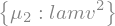
solve_tadpoles evaluates V on the vacuum, differentiates with respect to each registered VEV (∂V/∂v = 0), solves for mu2, and registers the solution on the InternalParameter — mu2.expr becomes lam*v**2. Every later stage (mass matrices, the physical Lagrangian, UFO export) automatically substitutes it.

Scalar masses come from the Hessian of V at the vacuum.

tadpole_solution = model.solve_tadpoles([mu2])
tadpole_solution

h, G0 = sp.Symbol("H0_r", real=True), sp.Symbol("H0_i", real=True)
m_h_squared = model.mass_matrix([h])[0, 0]
m_h_squared

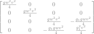
6. Gauge-boson masses and the Weinberg rotation

Gauge-boson masses come from the kinetic sector evaluated on the vacuum (scalars are constant there, so all ∂_μ terms vanish and only the g²v²·(gauge field)² piece survives). W1, W2 decouple from W3, B at this order; the (W3, B) block is the familiar singular matrix whose non-zero eigenvalue is m_Z² and whose zero eigenvalue is the photon.

W1, W2, W3 = SU2L.bosons().components
B = U1Y.bosons().components[0]
M2_gauge = model.gauge_mass_matrix([W1, W2, W3, B])
M2_gauge

A Rotation is new = R · old; register it and every later Lagrangian extraction rewrites the weak-basis fields for you.

• rotation_2x2(θ) is [[cosθ, sinθ], [−sinθ, cosθ]]; the minus sign on thetaW gives the textbook convention Z = cosθ_W W³ − sinθ_W B.

• kind="unitary" tells Rotation to use R† (not Rᵀ) as the inverse — needed for the complex combination W± = (W1 ∓ iW2)/√2.

Z, A = sp.symbols("Z A", real=True)
thetaW = sp.atan(g1.s / gw.s)
model.rotate(Rotation([W3, B], [Z, A], rotation_2x2(-thetaW)))

Wp, Wm = sp.symbols("Wp Wm")
U_charged = sp.Matrix([[1, -sp.I], [1, sp.I]]) / sp.sqrt(2)
model.rotate(Rotation([W1, W2], [Wp, Wm], U_charged, kind="unitary"))

"rotations registered:", len(model.rotations)

('rotations registered:', 2)

7. Extract the Feynman rules

What happens inside feynman_rules:

1. physical_lagrangian() takes the full L, applies the vacuum shift (H0 -> (v+h+iG0)/sqrt(2)), substitutes the tadpole solution for mu2, then applies every registered Rotation’s substitution dict — all lazily cached.

2. Since the kinetic sector has ∂_μ on every field, the result still contains PartialMu heads. These get Leibniz-expanded and sent to momentum space, ∂_μ φ → i·p(φ)·φ, tagging each leg with its own symbolic momentum p(φ).

3. conjugate_map rewrites conjugate(Gp) → the plain symbol Gm so the commuting-symbol extractor can see it as an ordinary field leg (Gp never got a VEV, so it stays a single complex physical field with its own antiparticle).

4. Every vertex gets the standard normalization i × coefficient × ∏(leg multiplicities)!.

Dict keys are in SymPy’s canonical sort order, not the order you write them in — look them up with a small helper (this is exactly what the test suite does).

Gp = H.components[0]
Gm, cmap = conjugate_pair(Gp, "Gm")
fields = [h, G0, Gp, Gm, Z, A, Wp, Wm]

rules = model.feynman_rules(fields, conjugate_map=cmap, simplifier=sp.simplify)

def rule(*flds):
    key = tuple(sorted(flds, key=lambda s: s.sort_key()))
    return rules[key]

f"{len(rules)} vertices extracted"

'38 vertices extracted'

print("hWW    =", rule(h, Wp, Wm))       # i g^2 v/2 = i g m_W
print("hhWW   =", rule(h, h, Wp, Wm))    # i g^2/2
print("hZZ    =", rule(h, Z, Z))         # i (g^2+g'^2) v/2

hWW    = I*gw**2*v/2
hhWW   = I*gw**2/2
hZZ    = I*v*(g1**2 + gw**2)/2

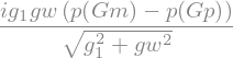
A momentum-dependent vertex — A G⁺ G⁻ (the scalar-QED photon coupling) — carries the antisymmetric combination p(Gp) − p(Gm), since it comes from the derivative (kinetic) term rather than the potential.

rule(A, Gp, Gm)

If you want typed objects instead of a flat dict (useful for UFO export or for grouping by vertex topology), use model.vertices(...) — same arguments, returns Vertex objects classified into the closed catalog SSS, SSSS, VSS, VVS, VVSS, VVV, VVVV, FFS, FFV by inspecting the spin content of each leg.

verts = model.vertices(fields, conjugate_map=cmap, simplifier=sp.simplify)
sorted({v.vertex_type for v in verts})

['SSS', 'SSSS', 'VSS', 'VVS', 'VVSS']

8. Pure-gauge self-couplings

Cubic/quartic pure-gauge self-couplings (γW⁺W⁻, W⁺W⁻W⁺W⁻, …) are not produced by feynman_rules — they come directly from the group’s structure constants, since their Lorentz structure is universal. You supply the mixing matrix U from adjoint components (W1, W2, W3) to the physical bosons (W+, W-, Z, A).

cubic_couplings returns the vertex coefficient directly: the cubic carries one derivative, so the i from ∂_μ → i p_μ cancels the Feynman-rule i. The i you see in g(A,W⁺W⁻) = i·e below therefore comes from the complex W± rotation U, not from a Feynman-rule factor — in a real basis the result is real, which is why the gluon comes out as ggg = -g_s. The quartic has no derivative, so there its i does survive and assemble_vvvv(..., feynman_rule=True) adds it.

Both return weak-basis values that carry the group factor (-g·f^{abc} for the cubic). For a broken group in the physical basis that factor is the coupling, but an unbroken group exports as one particle plus a colour tensor, so there the coupling must be colour-stripped — see export.ufo.vvvv.adjoint_vvv/adjoint_vvvv.

We print the magnitude to compare against the textbook value directly.

cw, sw = gw.s / sp.sqrt(gw.s**2 + g1.s**2), g1.s / sp.sqrt(gw.s**2 + g1.s**2)
U_mix = sp.Matrix([
    [1 / sp.sqrt(2), 1 / sp.sqrt(2), 0, 0],
    [sp.I / sp.sqrt(2), -sp.I / sp.sqrt(2), 0, 0],
    [0, 0, cw, sw],
])
triple = cubic_couplings(SU2L, physical=[Wp, Wm, Z, A], U=U_mix)

g_AWW = sp.simplify(triple[(A, Wp, Wm)])
g_ZWW = sp.simplify(triple[(Z, Wp, Wm)])
e = gw.s * sw   # = g sin(theta_W), the electric charge

print("g(A,W+,W-) =", g_AWW, " -> |g(A,W+,W-)| - e  =", sp.simplify(sp.Abs(g_AWW) - e))
print("g(Z,W+,W-) =", g_ZWW, " -> |g(Z,W+,W-)| - g*cos(theta_W) =",
      sp.simplify(sp.Abs(g_ZWW) - gw.s * cw))

g(A,W+,W-) = I*g1*gw/sqrt(g1**2 + gw**2)  -> |g(A,W+,W-)| - e  = 0
g(Z,W+,W-) = I*gw**2/sqrt(g1**2 + gw**2)  -> |g(Z,W+,W-)| - g*cos(theta_W) = 0

quartic = quartic_couplings(SU2L, physical=[Wp, Wm, Z, A], U=U_mix)
sp.simplify(quartic[(Wp, Wm, Wp, Wm)])   # WWWW quartic

9. Adding fermions: the SM lepton sector

Chiral fermions use a separate track from the scalar/gauge extractor above: a fermion sandwich ψ̄ Γ ψ is a c-number “atom”, not a product of commuting symbols, so it can’t go through the same Poly-based extractor.

• WeylFermion(name, reps=..., chirality=..., nflavors=...) declares a chiral multiplet; its gauge components are IndexedBase objects (one Indexed(base, flavor) per flavor), not plain Symbols.

• Bilinear(ψ̄[i], Γ, χ[j]) is the opaque atom representing a fermion sandwich, where Γ is a Dirac structure built from diracPL/diracPR/ DiracGamma(mu)*diracPL (see CONVENTIONS.md for the P_L=(1-γ₅)/2 convention).

• fermion_gauge_current(field, flavor_index) builds the interaction part of i ψ̄ γ^μ D_μ ψ for you — the analogue of Dmu for fermions.

Two things this section does not verify (documented gaps, not silent omissions): check_invariance()’s hermiticity check is skipped (not falsely failed) for any sector containing a Bilinear, since verifying [ψ̄₁Γψ₂]† = ψ̄₂Γ̄ψ₁ needs Dirac-conjugation identities not yet implemented — write + h.c. terms explicitly, as done below. And discrete-symmetry invariance checking (S3/ZN) doesn’t yet cover fermion multiplets either. Gauge invariance and mass-dimension checking of fermion terms, however, are fully implemented and exercised below.

Ll = WeylFermion("Ll", reps={SU2L: 2, U1Y: -sp.Rational(1, 2)},
                 chirality="L", nflavors=3, component_names=["nuL", "eL"])
eR = WeylFermion("eR", reps={U1Y: -1}, chirality="R", nflavors=3,
                 component_names=["eR"])

Ll.components, eR.components

The Yukawa Lagrangian, written by hand exactly like the potential was — a scalar factor times a Bilinear, plus its hermitian conjugate (built explicitly, since it can’t be auto-derived yet): L_Yuk = -Ye[i,j] L̄_i H e_R[j] + h.c., with the P_R sandwich carrying the right-handed projection and Ye a general flavor matrix.

i, j = sp.symbols("i j", integer=True)
Ye = sp.IndexedBase("Ye")
nuLbar, eLbar = Ll.bar_components
eRc, eRbar = eR.components[0], eR.bar_components[0]
Gp, H0 = H.components   # (re)bind: Gp was set in §7, H0 not yet named

LYuk = -(Ye[i, j] * Gp * Bilinear(nuLbar[i], diracPR, eRc[j])
         + Ye[i, j] * H0 * Bilinear(eLbar[i], diracPR, eRc[j]))
LYuk += -(sp.conjugate(Ye[i, j]) * sp.conjugate(Gp)
          * Bilinear(eRbar[j], diracPL, Ll.components[0][i])
          + sp.conjugate(Ye[i, j]) * sp.conjugate(H0)
          * Bilinear(eRbar[j], diracPL, Ll.components[1][i]))

current = fermion_gauge_current(Ll, i) + fermion_gauge_current(eR, i)
"Yukawa and gauge-current terms built"

'Yukawa and gauge-current terms built'

To add fermions to the model, build the complete Lagrangian (reusing the exact same DH, V expressions from §3) and construct one fresh Model with every field — this mirrors examples/sm_scalar_gauge.py, which does the same thing from the start rather than mutating the bosonic-only model from §4 in place. The already-found tadpole solution and Z/A/W± rotations are plain Python objects — reuse them directly.

L_full = Lagrangian()
L_full.add((dag(DH) * DH)[0], sector="kinetic")
L_full.add(-V, sector="potential")
L_full.add(LYuk, sector="yukawa")
L_full.add(current, sector="yukawa")

model_leptons = Model("SM-EW-leptons", gauge_groups=[SU2L, U1Y],
                      fields=[H, Ll, eR, SU2L.bosons(), U1Y.bosons()],
                      parameters=[gw, g1, v, lam, mu2], lagrangian=L_full)

report = model_leptons.check_invariance()
report

InvarianceReport(14 checks, OK)

model_leptons.solve_tadpoles([mu2])
for rot in model.rotations:      # reuse the Z/A and W+/W- rotations from §6
    model_leptons.rotate(rot)
"tadpoles solved, rotations applied"

'tadpoles solved, rotations applied'

Lepton mass matrix

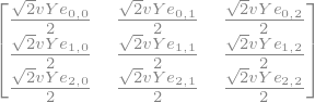
fermion_mass_matrix collects the coefficient of the Bilinear(ψ̄_a, Γ, χ_b) sandwich at the vacuum — the Lagrangian mass term is −ψ̄ M χ, so the returned matrix already has the right sign: M_e = Y_e v/√2.

M_e = fermion_mass_matrix(LYuk, eLbar, eRc, model_leptons.vacuum, 3, (i, j),
                          gamma=diracPR)
M_e

Fermion Feynman rules

model.physical_lagrangian(sector=...) applies the vacuum shift, tadpole solution, and every registered rotation to any sector — including "yukawa" — so the h/G0-lepton couplings and the already-rotated gauge currents come out of a single extract_fermion_vertices pass. Note the Yukawa term carries two flavor indices (Ye[i,j] connects the doublet’s flavor i to eR’s flavor j), while the gauge currents are flavor-diagonal (same index on both legs) — the lookup key must match.

Gm, cmap = conjugate_pair(Gp, "Gm")
boson_fields = [h, G0, Gp, Gm, Z, A, Wp, Wm]

LYuk_phys = model_leptons.physical_lagrangian(sector="yukawa").xreplace(cmap)
table = extract_fermion_vertices(LYuk_phys, boson_fields)

mu = sp.Symbol("mu", integer=True)
gammaL = DiracGamma(mu) * diracPL
gammaR = DiracGamma(mu) * diracPR
nuL, eL = Ll.components

def fermion_rule(bar, gamma, field, boson):
    coeff = table[(bar, gamma, field)][1][(boson,)]
    return sp.simplify(fermion_feynman_rule(coeff, gamma, (boson,)))

print("h  e_L e_R ->", fermion_rule(eLbar[i], diracPR, eRc[j], h))
print("W+ nu  e   ->", fermion_rule(nuLbar[i], gammaL, eL[i], Wp))
print("Z  e_L e_L ->", fermion_rule(eLbar[i], gammaL, eL[i], Z))
print("Z  e_R e_R ->", fermion_rule(eRbar[i], gammaR, eRc[i], Z))
print("A  e_L e_L ->", fermion_rule(eLbar[i], gammaL, eL[i], A))
print("A  e_R e_R ->", fermion_rule(eRbar[i], gammaR, eRc[i], A))

h  e_L e_R -> -sqrt(2)*I*Ye[i, j]*PR/2
W+ nu  e   -> sqrt(2)*I*gw*gamma(mu)*PL/2
Z  e_L e_L -> I*(g1**2 - gw**2)*gamma(mu)*PL/(2*sqrt(g1**2 + gw**2))
Z  e_R e_R -> I*g1**2*gamma(mu)*PR/sqrt(g1**2 + gw**2)
A  e_L e_L -> -I*g1*gw*gamma(mu)*PL/sqrt(g1**2 + gw**2)
A  e_R e_R -> -I*g1*gw*gamma(mu)*PR/sqrt(g1**2 + gw**2)

The h e_L e_R rule, specialized to a single flavor with Y_e = √2 m_ℓ/v (the diagonal-mass convention), reduces to the pinned value −i m_ℓ/v · P_R (+ h.c.) — and the W⁺νe/Z/γ couplings above match i g/√2 · γ^μP_L, the g_Z(T³−Qs²_W) pattern, and ∓ie respectively, all cross-checked in tests/test_fermion_sector.py (which also covers diagonalize_svd/diagonalize_takagi for 3-generation mass matrices and a toy type-I seesaw — not repeated here).

m_ell = sp.Symbol("m_ell", positive=True)
hll_coeff = table[(eLbar[i], diracPR, eRc[j])][1][(h,)]
hll_rule = fermion_feynman_rule(hll_coeff, diracPR, (h,))
sp.simplify(hll_rule.subs(Ye[i, j], sp.sqrt(2) * m_ell / v.s))

10. Output: LaTeX tables and UFO export

latex_feynman_table produces a ready-to-paste \begin{array} table.

preview = {k: rules[k] for k in list(rules)[:4]}
print(latex_feynman_table(preview))

\begin{array}{|c|c|}
\hline
\textbf{Interaction} & \textbf{Coefficient} \\
\hline
$A A Gm Gp$ & $\frac{2 i g_{1}^{2} gw^{2}}{g_{1}^{2} + gw^{2}}$ \\
\hline
$A Gm Gp Z$ & $\frac{i g_{1} gw \left(- g_{1}^{2} + gw^{2}\right)}{g_{1}^{2} + gw^{2}}$ \\
\hline
$A Gm H_{0 i} Wp$ & $- \frac{g_{1} gw^{2}}{2 \sqrt{g_{1}^{2} + gw^{2}}}$ \\
\hline
$A Gm H_{0 r} Wp$ & $\frac{i g_{1} gw^{2}}{2 \sqrt{g_{1}^{2} + gw^{2}}}$ \\
\hline
\end{array}

For a MadGraph-importable model directory, use feynlag.export.ufo.write_ufo(...) — it needs a UFOParticle spec per physical field (PDG code, spin, mass parameter name, color, charge). See tests/test_ufo_export.py for a complete worked call, including a numeric round-trip check that the exported hWW coupling evaluates to i g² v/2.

11. Extending the SM: writing a BSM model

Every BSM model follows exactly the pipeline above; the only things that change are what you declare in §1–§3. Worked templates already live in examples/thdm.py (a second Higgs doublet, softly-broken Z₂) and examples/thdm_s3.py (a discrete S₃ flavor symmetry across three doublets) — read them alongside this checklist:

1. New fields: declare extra Scalar/Fermion/GaugeBosons with their representations under your (possibly extended) symmetry groups. Extra gauge groups are just more SU2/U1/SU3 objects passed to gauge_groups=[...]; a gauged extra U(1)' is created exactly like U1Y above.

2. New symmetries: for a discrete symmetry (softly-broken Z₂ picking out Yukawa alignment in a 2HDM, or an S₃ flavor symmetry across three doublets), instantiate ZN(name, N) or S3(), then group.assign(irrep, *fields). S3.doublet_product(...) gives you the 2⊗2 = 1⊕1'⊕2 Clebsch–Gordan contractions to build invariant terms without doing the group theory by hand — thdm_s3.py builds its entire potential this way.

3. Extend the potential/Yukawas: write the new invariant contractions (dag(H1)*H2.mat, CG products, …) and add them to a Lagrangian sector. Call model.check_invariance() immediately — a forbidden term (wrong representation, missing + h.c., wrong discrete charge) fails loudly instead of silently producing wrong Feynman rules downstream.

4. VEVs on every scalar that gets one, then solve_tadpoles([...]) for as many mass parameters as you have independent tadpole conditions. If the system is over-constrained (more tadpole equations than free mass parameters — the thdm_s3.py case), that’s physical: it’s forcing a vacuum alignment, visible as a residual condition on the VEV ratios after solving the others (exactly how thdm_s3.py recovers the √3 alignment).

5. Mass matrices grow with the field content: model.mass_matrix([...]) accepts any list of same-block fluctuation symbols — a 3×3 CP-even block for a 3HDM works identically to the SM’s 1×1 above. For blocks too large to diagonalize in closed form (≥3×3 symbolic), don’t call sp.Matrix.eigenvects directly; either parametrize a rotation and solve the off-diagonal conditions numerically at benchmark points, or export to UFO and diagonalize numerically downstream.

6. Register every new rotation the same way as alpha/beta in thdm.py’s CP-even block.

7. Extract vertices exactly as in §7, just with a longer fields list. Chiral fermions use a parallel “bilinear” track (feynlag.Bilinear, fermion_gauge_current, extract_fermion_vertices) since a fermion sandwich is a c-number atom, not a product of commuting symbols — §9 above works through the full SM-lepton case (Yukawa, gauge currents, mass matrix, Feynman rules, including how check_invariance() now covers fermion gauge invariance and mass dimension); see tests/test_fermion_sector.py for the 3-generation diagonalize_svd/diagonalize_takagi and seesaw pieces not repeated there.

The invariant is: nothing about Model, check_invariance, solve_tadpoles, mass_matrix, rotate, or feynman_rules is SM-specific — they operate purely on whatever fields, symmetries, and Lagrangian terms you declared. Growing the model is additive, not a rewrite. As a taste of step 1–2, here is the declaration half of a second Higgs doublet (the full potential and pipeline is in thdm.py):

H2 = Scalar("H2", reps={SU2L: 2, U1Y: sp.Rational(1, 2)},
            component_names=["H2p", "H20"])
v2 = ExternalParameter("v2", 246.0 * 0.31, positive=True, unit_dim=1)
H2.expand_vev({H2.components[1]: v2})

# a new SU(2)xU(1)-invariant mixed bilinear, available for the potential:
H1dH2 = (dag(H) * H2.mat)[0]
H1dH2