3HDM with S₃ flavor symmetry: forcing the vacuum, not tuning it

A generic three-Higgs-doublet potential has dozens of independent quartic couplings — far too many to be predictive. One standard way to cut that down is to impose a discrete flavor symmetry on the scalar sector: pick a finite group, assign the doublets to its representations, and keep only the quartic invariants that group theory allows.

This notebook builds the simplest non-abelian example: \(S_3\), the permutation group on 3 objects, with \((H_1, H_2)\) forming its 2-dimensional irrep and a third doublet \(H_S\) sitting in the trivial singlet. It follows examples/thdm_s3.py step by step, showing two things no earlier feynlag tutorial needed:

1. Finite discrete-symmetry invariance. Every gauge check in prior tutorials linearizes the transformation at \(\alpha=0\) (a continuous Lie group). \(S_3\) has no such infinitesimal neighborhood of the identity — feynlag instead applies the group’s exact, finite substitution and checks the Lagrangian term-by-term for literal equality.

2. A vacuum that isn’t free to choose. With three VEVs (\(v_1, v_2, v_S\)) but an \(S_3\)-covariant potential that only has two independent mass parameters (\(\mu_0^2,\mu_1^2\)) to absorb tadpole conditions, the third condition becomes a real constraint. Solving it doesn’t tune a free ratio — it forces \(v_1/v_2\) to a fixed value.

Along the way we also see the \(S_3\) Clebsch–Gordan decomposition \(2\otimes2 = 1\oplus1'\oplus2\) that the potential is built from, the resulting CP-even, pseudoscalar and charged mass matrices, and — following the literature model this potential is drawn from — a geometric rotation ansatz that diagonalizes them into seven physical scalar masses.

Assumed background: the Higgs mechanism / spontaneous gauge symmetry breaking, Goldstone’s theorem, and enough Lie-group representation theory to know what a tensor-product (Clebsch–Gordan) decomposition is — the kind of material a first QFT course plus a group-theory-for-physicists chapter covers. If tensor products/irreps are new, SUN_Groups_Tutorial.ipynb builds that machinery up from scratch first (for continuous groups; \(S_3\) here is discrete, but the tensor-product idea is the same). The library-specific machinery this notebook exercises (S3, Model, Rotation, …) is documented in docs/manual/declaration.md and docs/manual/ssb.md.

Notation used throughout this notebook:

Symbol	Meaning
\(H_1,H_2,H_S\)	the three \(SU(2)_L\times U(1)_Y\) Higgs doublets (\(H_1,H_2\) in the \(S_3\) 2, \(H_S\) in the 1)
\(v_1,v_2,v_S\)	their vacuum expectation values
\(\lambda_1,\ldots,\lambda_8\)	the eight \(S_3\)-invariant quartic couplings (§2 table)
\(\mu_0^2,\mu_1^2\)	the singlet/doublet-sector mass² parameters
\(M_S^2,\,M_A^2,\,M_C^2\)	the CP-even, pseudoscalar (CP-odd) and charged \(3\times3\) mass-squared matrices
\(R(\varphi,\theta)\)	the geometric (coupling-independent) rotation fixed by the vacuum direction alone
\(\alpha\)	the one genuinely dynamical mixing angle, needed only for the CP-even sector
\(h_0,H_1,H_2\)	the three physical CP-even scalars
\(A_1,A_2\)	the two physical pseudoscalars (the third pseudoscalar direction is the \(Z\)’s Goldstone)
\(H_1^\pm,H_2^\pm\)	the two physical charged scalars (the third charged direction is the \(W^\pm\)’s Goldstone)

Keep this table in view — the notebook builds every one of these from scratch, in this order.

1. Symmetries, parameters, fields

\(S_3\) has three irreducible representations:

• \(\mathbf{1}\) — trivial: every group element acts as \(+1\).

• \(\mathbf{1'}\) — the sign representation: the 3-cycle acts as \(+1\), the transposition as \(-1\).

• \(\mathbf{2}\) — a genuine 2-dimensional (real, orthogonal) doublet: feynlag’s S3 represents the 3-cycle generator as a \(2\pi/3\) rotation matrix and the transposition generator as a reflection \(\mathrm{diag}(1,-1)\).

s3.assign(irrep, *fields) below registers which fields sit in which irrep and builds, from those generator matrices, an explicit finite substitution map (one linear combination of components per group generator) — this is what check_discrete_invariance later applies exactly, in contrast to the \(O(\alpha)\) linearized check every gauge symmetry in this library uses.

We also declare the usual electroweak gauge sector (\(SU(2)_L\times U(1)_Y\)) alongside \(S_3\) — the potential must satisfy both symmetries at once.

import sympy as sp
from IPython.display import display
sp.init_printing()

from feynlag import (
    ExternalParameter, InternalParameter, Lagrangian, Model, S3, SU2,
    Scalar, U1, check_discrete_invariance, dag,
)

gw = ExternalParameter("g_w", 0.6535, positive=True)
g1 = ExternalParameter("g_1", 0.3580, positive=True)
SU2L, U1Y = SU2("SU2L", coupling=gw), U1("U1Y", coupling=g1)
s3 = S3()

v1 = ExternalParameter("v_1", 200.0, positive=True, unit_dim=1)
v2 = ExternalParameter("v_2", 115.0, positive=True, unit_dim=1)
vS = ExternalParameter("v_S", 80.0, positive=True, unit_dim=1)
lams = {k: ExternalParameter(f"lambda_{k}", 0.05 * k) for k in range(1, 9)}
mu0sq = InternalParameter("mu0sq", unit_dim=2)
mu1sq = InternalParameter("mu1sq", unit_dim=2)

\(v_1,v_2,v_S=200,115,80\) GeV aren’t arbitrary: they’re chosen so that \(\sqrt{v_1^2+v_2^2+v_S^2}\approx246\) GeV, the single familiar SM Higgs VEV — [GomezBock21]’s Eq. (8) constraint. Three doublets, one combined scale.

Before wiring up real fields, let’s see the \(2\otimes2\) Clebsch–Gordan decomposition on abstract symbols — S3.doublet_product returns the three channels the tensor product of two doublets splits into.

a1, a2, b1, b2 = sp.symbols("a1 a2 b1 b2")
cg = s3.doublet_product((a1, a2), (b1, b2))
cg

{'1': a1*b1 + a2*b2, '1p': a1*b2 - a2*b1, '2': (a1*b1 - a2*b2, -a1*b2 - a2*b1)}

So \(2\otimes2 = 1\oplus1'\oplus2\): a singlet (\(a_1b_1+a_2b_2\)), a pseudo-singlet (\(a_1b_2-a_2b_1\)), and — since a doublet’s tensor square must contain another doublet — a second copy of the 2 itself. We’ll reuse these exact three combinations below, applied not to raw field components but to the gauge-invariant bilinears \(H_i^\dagger H_j\).

2. Building the \(S_3\)-covariant potential from Clebsch–Gordan invariants

\(H_1, H_2, H_S\) are three ordinary \(SU(2)_L\times U(1)_Y\) Higgs doublets. s3.assign("2", H1, H2) puts \((H_1,H_2)\) in the doublet irrep; s3.assign("1", HS) puts \(H_S\) in the trivial singlet.

def doublet(name):
    return Scalar(name, reps={SU2L: 2, U1Y: sp.Rational(1, 2)},
                  component_names=[f"{name}p", f"{name}0"])

H1, H2, HS = doublet("H_1"), doublet("H_2"), doublet("H_S")
s3.assign("2", H1, H2)
s3.assign("1", HS)

H1.expand_vev({H1.components[1]: v1})
H2.expand_vev({H2.components[1]: v2})
HS.expand_vev({HS.components[1]: vS})

\[\displaystyle H_{S} = (H_{Sp}, H_{S0})\]

bra(a, b) builds the \(SU(2)_L\times U(1)_Y\)-invariant bilinear \(a^\dagger b\). The doublet-index CG formulas from above apply directly to these bilinears, with \((a_1,a_2)=(H_1^\dagger,H_2^\dagger)\) on the bra side and \((b_1,b_2)=(H_1,H_2)\) on the ket side: \(a_1b_1\to H_1^\dagger H_1\), \(a_1b_2\to H_1^\dagger H_2\), and so on.

def bra(a, b):
    return (dag(a) * b.mat)[0]

x11, x22 = bra(H1, H1), bra(H2, H2)
x12, x21 = bra(H1, H2), bra(H2, H1)
s1, s2 = bra(HS, H1), bra(HS, H2)
sss = bra(HS, HS)

inv1 = x11 + x22          # the '1' channel:  a1*b1 + a2*b2
inv1p = x12 - x21         # the '1\'' channel: a1*b2 - a2*b1
d2 = (x11 - x22, -(x12 + x21))   # the '2' channel

display(inv1)
display(inv1p)
display(d2)

\(H_S\) enters the potential through its own doublet of bilinears, \((s_1,s_2)=(H_S^\dagger H_1,\,H_S^\dagger H_2)\), which transforms exactly like \((H_1,H_2)\) under \(S_3\). Contracting this doublet with itself, or with the \((H_1,H_2)\) doublet channel d2, gives two more singlet invariants — both need an explicit \(+\text{h.c.}\) since neither combination is manifestly real on its own.

lam4_term = s1 * d2[0] + s2 * d2[1]
lam4_term += sp.conjugate(lam4_term)     # (HS†H)_2 ⊗ (H†H)_2 → 1, + h.c.

lam7_term = s1**2 + s2**2
lam7_term += sp.conjugate(lam7_term)     # (HS†H)_2 ⊗ (HS†H)_2 → 1, + h.c.

display(lam4_term)
display(lam7_term)

All 8 quartic couplings are now S₃-invariant combinations built from inv1, inv1p, d2, lam4_term, lam7_term, sss:

Coupling	CG channel	Term	Role
\(\lambda_1\)	\(1\otimes1\)	\((H_1^\dagger H_1+H_2^\dagger H_2)^2\)	ordinary doublet-sector quartic
\(\lambda_2\)	\(1'\otimes1'\)	\((H_1^\dagger H_2-H_2^\dagger H_1)^2\)	pseudo-singlet quartic
\(\lambda_3\)	\(2\otimes2\to1\)	\(d_2\cdot d_2\)	doublet-channel self-contraction
\(\lambda_4\)	\((H_S^\dagger H)_2\otimes(H^\dagger H)_2\to1\), + h.c.	\(s\cdot d_2\) + h.c.	singlet–doublet mixed quartic
\(\lambda_5\)	\(1\otimes1\)	\((H_S^\dagger H_S)(H_1^\dagger H_1+H_2^\dagger H_2)\)	portal-like singlet×doublet-norm coupling
\(\lambda_6\)	\(2\otimes\bar2\to1\)	\(s_1(H_1^\dagger H_S)+s_2(H_2^\dagger H_S)\)	\(|s_1|^2+|s_2|^2\)-type cross term
\(\lambda_7\)	\((H_S^\dagger H)_2\otimes(H_S^\dagger H)_2\to1\), + h.c.	\(s_1^2+s_2^2\) + h.c.	CP-sensitive; needs + h.c. to be Hermitian
\(\lambda_8\)	\(1\otimes1\)	\((H_S^\dagger H_S)^2\)	pure singlet quartic

plus a mass term for each \(S_3\) singlet sector, \(\mu_1^2(H_1^\dagger H_1+H_2^\dagger H_2)\) and \(\mu_0^2 H_S^\dagger H_S\).

l = {k: p.s for k, p in lams.items()}
V = (mu1sq.s * inv1 + mu0sq.s * sss
     + l[1] * inv1**2 + l[2] * inv1p**2
     + l[3] * (d2[0]**2 + d2[1]**2)
     + l[4] * lam4_term
     + l[5] * sss * inv1
     + l[6] * (s1 * bra(H1, HS) + s2 * bra(H2, HS))
     + l[7] * lam7_term
     + l[8] * sss**2)

L = Lagrangian().add(-V, sector="potential")

3. Assemble the model and check invariance

Everything above was built from gauge-invariant bilinears and \(S_3\) Clebsch–Gordan combinations by hand — but nothing has actually verified gauge or \(S_3\) invariance yet. Model.check_invariance() checks every term against both gauge_groups and discrete_groups at once.

model = Model("3HDM-S3", gauge_groups=[SU2L, U1Y], discrete_groups=[s3],
              fields=[H1, H2, HS],
              parameters=[gw, g1, v1, v2, vS, mu0sq, mu1sq,
                          *lams.values()],
              lagrangian=L)

report = model.check_invariance()
print("invariant:", report.ok)
if not report.ok:
    print(report.failures)

invariant: True

In plain terms: every coupling written into \(V\) is simultaneously allowed — there’s no hidden tension between the gauge and \(S_3\) symmetries that would force some \(\lambda_k\) to vanish.

What if a term weren’t \(S_3\)-invariant? Take, for instance, \((H_S^\dagger H_1)(H_1^\dagger H_1) + \text{h.c.}\) — it singles out \(H_1\) without pairing it with the matching \(H_2\) combination the doublet structure requires. check_discrete_invariance catches this directly, without needing a full Model.

bad = (dag(HS) * H1.mat)[0] * (dag(H1) * H1.mat)[0]
bad = bad + sp.conjugate(bad)

ok, _ = check_discrete_invariance(bad, s3)
print("forbidden term is S3-invariant?", ok)

forbidden term is S3-invariant? False

4. Tadpoles and the forced \(\sqrt3\) vacuum alignment

There are three VEVs (\(v_1,v_2,v_S\)) but the \(S_3\)-covariant potential only has two independent mass parameters (\(\mu_0^2,\mu_1^2\)) free to absorb tadpole conditions. Solving the \(v_2\) and \(v_S\) conditions for \(\mu_0^2,\mu_1^2\) and substituting into the \(v_1\) condition therefore leaves a genuine constraint on \(v_1,v_2\) alone — not an identity.

tadpoles = model.tadpoles()
t1, t2, tS = tadpoles[v1.s], tadpoles[v2.s], tadpoles[vS.s]

sol = sp.solve([sp.Eq(t2, 0), sp.Eq(tS, 0)], [mu0sq.s, mu1sq.s], dict=True)[0]
residual = sp.factor(sp.expand(t1.subs(sol)))
print("residual v1-tadpole condition:")
display(residual)

residual v1-tadpole condition:

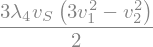
The residual factors as \(\propto v_S(3v_1^2 - v_2^2)\): since \(v_S\neq0\), the only way to satisfy all three tadpole conditions simultaneously is \(v_1^2 = v_2^2/3\) — a fixed ratio, not a free parameter. (docs/manual/ssb.md frames this as a structural consequence of the CG structure, not a coincidence of the numeric benchmark point; the declaration.md chapter notes that feynlag’s real-orthogonal \(S_3\) basis swaps which doublet component the literature’s \(v_1=\sqrt3\,v_2\) convention refers to — the ratio squared is the basis-independent statement.)

This exact relation was independently derived in the literature model this potential is drawn from: [GomezBock21] M. Gómez-Bock, M. Mondragón, A. Pérez-Martínez, “Scalar and gauge sectors in the 3-Higgs Doublet Model under the S₃-symmetry”, Eur. Phys. J. C 81, 942 (2021), arXiv:2102.02800, doi:10.1140/epjc/s10052-021-09731-3 — their Eq. (13) tadpole solution is exactly \(v_1^2=3v_2^2\) (their \(v_1,v_2\); the basis swap above is what turns this into our \(v_1^2=v_2^2/3\)).

v1_solutions = sp.solve(sp.Eq(residual, 0), v1.s)
print("v1 solutions:", v1_solutions)
for s_v1 in v1_solutions:
    ratio_sq = sp.simplify((s_v1 / v2.s) ** 2)
    print("  (v1/v2)^2 =", ratio_sq)

v1 solutions: [sqrt(3)*v_2/3]
  (v1/v2)^2 = 1/3

In plain terms: naively, three VEVs minus three tadpole conditions should still leave one free ratio to fit experimentally — instead the \(S_3\) structure removes it. The model has one fewer free continuous parameter than the field content alone would suggest.

5. CP-even mass matrix on the aligned vacuum

Imposing the alignment and re-solving the two mass parameters consistently, the \(v_1\) tadpole condition is now automatically satisfied — confirming the alignment is exactly what’s needed, not an approximation.

align = {v1.s: v2.s / sp.sqrt(3)}

sol2 = sp.solve([sp.Eq(tadpoles[v2.s].subs(align), 0),
                 sp.Eq(tadpoles[vS.s].subs(align), 0)],
                [mu0sq.s, mu1sq.s], dict=True)[0]

print("v1 tadpole after alignment + resolving mu0sq, mu1sq:",
      sp.simplify(tadpoles[v1.s].subs(align).subs(sol2)))

v1 tadpole after alignment + resolving mu0sq, mu1sq: 0

Model.mass_matrix takes the real CP-even fluctuations (expand_vev’s auto-generated {name}0_r symbols) and returns \(\partial^2V/\partial\phi_i\partial\phi_j\) evaluated on the vacuum, with any cached tadpole solutions applied automatically.

h = [sp.Symbol(f"{n}0_r", real=True) for n in ("H_1", "H_2", "H_S")]
M = model.mass_matrix(h).subs(sol2).subs(align)
M = M.applyfunc(lambda e: sp.simplify(sp.expand(e)))
M

print("symmetric:", sp.simplify(M - M.T) == sp.zeros(3, 3))
print("nonzero diagonal:", M[0, 0] != 0 and M[1, 1] != 0 and M[2, 2] != 0)

symmetric: True
nonzero diagonal: True

6. The other two scalar sectors: pseudoscalar and charged mass matrices

thdm_s3.py’s potential V was written from full doublet bilinears (bra, dag(a)*b.mat) — it already implicitly contains the charged (\(H_1^\pm,H_2^\pm,H_S^\pm\)) and imaginary neutral (pseudoscalar) pieces of every field, even though only the real neutral fluctuations (_r symbols) have been differentiated so far. No new Lagrangian terms are needed to get the other two sectors, just two more second-derivative matrices:

• Pseudoscalar (\(M_A^2\)): the same Model.mass_matrix used for the CP-even sector, applied to expand_vev’s imaginary (_i) fluctuation symbols instead of the real ones.

• Charged (\(M_C^2\)): Model.mass_matrix(..., charged=True), which differentiates \(\partial^2V/\partial\bar\phi_i\partial\phi_j\) via a Dummy-conjugate trick (SymPy can’t differentiate w.r.t. conjugate(φ) directly) — this one takes the raw charged component symbols (H1.components[0], etc.), not fluctuation symbols, since a charged field never gets a VEV and so never had _r/_i symbols generated for it.

hi = [sp.Symbol(f"{n}0_i", real=True) for n in ("H_1", "H_2", "H_S")]
M_A = model.mass_matrix(hi).subs(sol2).subs(align)
M_A = M_A.applyfunc(lambda e: sp.simplify(sp.expand(e)))

hc = [H1.components[0], H2.components[0], HS.components[0]]
M_C = model.mass_matrix(hc, charged=True).subs(sol2).subs(align)
M_C = M_C.applyfunc(lambda e: sp.simplify(sp.expand(e)))

print("M_A symmetric:", sp.simplify(M_A - M_A.T) == sp.zeros(3, 3))
print("M_C symmetric:", sp.simplify(M_C - M_C.T) == sp.zeros(3, 3))
display(M_A)
display(M_C)

M_A symmetric: True
M_C symmetric: True

7. The Gómez-Bock–Mondragón–Pérez-Martínez rotation ansatz

[GomezBock21] (full citation above) diagonalizes all three sectors with a rotation built purely from the geometry of the vacuum. Writing \(v_1=v\cos\varphi\sin\theta\), \(v_2=v\sin\varphi\sin\theta\), \(v_S=v\cos\theta\) (their Eq. 21) — i.e. \(\varphi,\theta\) are just the angles the VEV vector makes in \((v_1,v_2,v_S)\)-space — their Eq. 25–29 rotation is

\[\begin{split}R(\varphi,\theta)=\begin{pmatrix}\sin\theta\cos\varphi&-\sin\varphi&-\cos\theta\cos\varphi\\\sin\theta\sin\varphi&\cos\varphi&-\cos\theta\sin\varphi\\\cos\theta&0&\sin\theta\end{pmatrix}.\end{split}\]

Nothing here depends on the potential’s couplings — it’s fixed the moment the vacuum direction is known. We build it directly from feynlag’s own \(v_1,v_2,v_S\) (no basis translation needed — tested below against the swapped assignment too, which does not diagonalize; this direct one does).

v12 = sp.sqrt(v1.s**2 + v2.s**2)
vtot = sp.sqrt(v1.s**2 + v2.s**2 + vS.s**2)
cphi, sphi = v1.s / v12, v2.s / v12
cth, sth = vS.s / vtot, v12 / vtot

R = sp.Matrix([
    [sth * cphi, -sphi, -cth * cphi],
    [sth * sphi,  cphi, -cth * sphi],
    [cth,          0,    sth],
])
R = sp.simplify(R.subs(align))
R

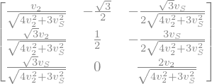
Checking the expressions are right (not assuming): apply \(R^TM_AR\) and \(R^TM_CR\) and look at which entries are identically zero, for arbitrary \(\lambda_1,\ldots,\lambda_8\) — no numbers substituted yet.

def zero_pattern(D):
    return [[bool(sp.simplify(D[i, j]) == 0) for j in range(3)] for i in range(3)]

D_A = sp.simplify(R.T * M_A * R)
D_C = sp.simplify(R.T * M_C * R)

print("D_A = R^T M_A R zero pattern:")
for row in zero_pattern(D_A):
    print("  ", row)
print("D_C = R^T M_C R zero pattern:")
for row in zero_pattern(D_C):
    print("  ", row)

print("\nGoldstone eigenvalues (should be exactly 0):", D_A[0, 0], D_C[0, 0])
print("\npseudoscalar physical mass^2 formulas:")
display(D_A[1, 1])
display(D_A[2, 2])
print("charged physical mass^2 formulas:")
display(D_C[1, 1])
display(D_C[2, 2])

D_A = R^T M_A R zero pattern:
   [True, True, True]
   [True, False, True]
   [True, True, False]
D_C = R^T M_C R zero pattern:

   [True, True, True]
   [True, False, True]
   [True, True, False]

Goldstone eigenvalues (should be exactly 0): 0 0

pseudoscalar physical mass^2 formulas:

charged physical mass^2 formulas:

\(R\) exactly, fully diagonalizes both sectors — for any couplings, not just the benchmark point — with one eigenvalue identically zero (the Goldstone boson eaten by \(Z\) and \(W^\pm\) respectively) and two compact closed-form mass² formulas. This matches [GomezBock21]’s Eq. 30–33: the pseudoscalar and charged sectors need no mixing angle beyond this one geometric rotation, because it’s fixed entirely by the Goldstone theorem — gauge symmetry alone, nothing dynamical about the potential.

Does the same trick fully diagonalize the CP-even sector M from §5?

In plain terms: two of the twelve real scalar degrees of freedom the three doublets started with are exactly massless before any dynamics is switched on at all — pure kinematics from the Goldstone theorem, later eaten as the longitudinal modes of \(Z\) and \(W^\pm\), not a coincidence of these particular \(\lambda_k\).

D_S = sp.simplify(R.T * M * R)
print("D_S = R^T M R zero pattern:")
for row in zero_pattern(D_S):
    print("  ", row)
D_S

D_S = R^T M R zero pattern:

   [False, True, False]
   [True, False, True]
   [False, True, False]

Only one state decouples this time (row/column 1 — the analogue of [GomezBock21]’s \(h_0\), with the compact closed form \(m_{h_0}^2=3\sqrt3\,\lambda_4v_2v_S\), independent of every other coupling including \(\lambda_8\)). The remaining \((0,2)\) block is not diagonal — a genuine, coupling-dependent mixing survives. This is the qualitative difference [GomezBock21] report: the CP-even sector needs a second, dynamical mixing angle (their \(\alpha\), Eq. 36) that the Goldstone-protected pseudoscalar/charged sectors don’t.

8. Finishing the CP-even sector: the leftover \(2\times2\) block

This is exactly the shape feynlag.vacuum.diagonalize.solve_mixing_angle_2x2 / diagonalize_orthogonal_2x2 already handles — the same tool examples/thdm.py uses to diagonalize the plain 2HDM’s \(2\times2\) CP-even matrix, reused here on the block left over after the geometric rotation above.

from feynlag import solve_mixing_angle_2x2, diagonalize_orthogonal_2x2

block = sp.Matrix([[D_S[0, 0], D_S[0, 2]], [D_S[2, 0], D_S[2, 2]]])
theta_expr, tan2theta = solve_mixing_angle_2x2(block)
print("tan(2 theta) is a closed form of length", len(str(tan2theta)),
      "characters (long, but a genuine analytic formula — unlike the raw",
      "cubic-root diagonalization of the full 3x3, this 2x2 reduction stays",
      "closed-form)")

h_a, h_b, H_1, H_2 = sp.symbols("h_a h_b H_1 H_2", real=True)
rot = diagonalize_orthogonal_2x2(block, [h_a, h_b], [H_1, H_2])
rot.angle_relation

tan(2 theta) is a closed form of length 707 characters (long, but a genuine analytic formula — unlike the raw cubic-root diagonalization of the full 3x3, this 2x2 reduction stays closed-form)

707 characters is unreadable as one blob — but it’s a sum of terms each proportional to a single \(\lambda_k\). Factoring groups them, which at least makes the structure (which couplings enter, and how) legible even though the full expression stays long.

tan2theta.factor()

9. Physical spectrum at a benchmark point

Substituting numeric values (each parameter’s own declared ExternalParameter.value, as in previous benchmark checks) into the original λ = 0.05·k demonstration point shows the same lesson as before, now for all three sectors at once — solving the tadpoles only guarantees a stationary point, and the mass matrices are the second-derivative stability test.

lam_syms = [lams[k].s for k in range(1, 9)]
spectrum_exprs = [D_S[1, 1], D_S[0, 0], D_S[0, 2], D_S[2, 2],
                  D_A[1, 1], D_A[2, 2], D_C[1, 1], D_C[2, 2]]
spectrum_fn = sp.lambdify(lam_syms + [v2.s, vS.s], spectrum_exprs, "math")

def block_eigs(a, b, c):
    # real symmetric 2x2: discriminant (a-c)^2 + 4b^2 is never negative
    tr, det = a + c, a * c - b * b
    root = (tr**2 - 4 * det) ** 0.5
    return (tr + root) / 2, (tr - root) / 2

def spectrum(lam_values, v2_val, vS_val):
    h0, a, b, c, A1, A2, Hp1, Hp2 = spectrum_fn(*lam_values, v2_val, vS_val)
    H1m, H2m = block_eigs(a, b, c)
    return dict(h0=h0, H1=H1m, H2=H2m, A1=A1, A2=A2, Hpm1=Hp1, Hpm2=Hp2)

spectrum(...) turns any set of couplings into all seven physical mass² values at once, reusing the closed forms just derived. Now evaluate it at the same “democratic” \(\lambda_k=0.05k\) point used throughout the notebook so far.

naive_lams = [0.05 * k for k in range(1, 9)]
naive = spectrum(naive_lams, v2.value, vS.value)
print("naive benchmark mass^2 (GeV^2):", {k: round(v, 2) for k, v in naive.items()})
print("negative directions:", [k for k, v in naive.items() if v < 0])

naive benchmark mass^2 (GeV^2): {'h0': 9560.92, 'H1': 14214.63, 'H2': -2301.34, 'A1': -7985.04, 'A2': -12834.08, 'Hpm1': -3178.38, 'Hpm2': -8027.42}
negative directions: ['H2', 'A1', 'A2', 'Hpm1', 'Hpm2']

In plain terms: a negative mass² here doesn’t mean an imaginary-mass particle — it flags a direction in which the potential curves downward at this point. This benchmark sits on a saddle/hilltop of \(V\), not in a valley, in five of the seven directions.

Five of the seven directions are tachyonic at this naive, “democratic” benchmark. [GomezBock21] face exactly this problem at scale — their Section 3.4 scans \(\mathcal O(10^{11})\) random points over the eight self-couplings and keeps only the ones passing unitarity and stability constraints before ever reporting a mass. We do the same thing here, just at notebook scale: a small random scan over \(\lambda_1,\ldots,\lambda_8\) (same \(v_2,v_S\)) for the first point where all seven mass² come out positive.

import random

rng = random.Random(7)
stable = None
for trial in range(500_000):
    lam_values = [rng.uniform(0.0, 1.5) for _ in range(8)]
    spec = spectrum(lam_values, v2.value, vS.value)
    if all(m2 > 0 for m2 in spec.values()):
        stable = (lam_values, spec)
        break

The scan above just stops at the first point where all seven mass² come out positive — a stand-in, at notebook scale, for [GomezBock21]’s \(\mathcal O(10^{11})\)-point stability/unitarity scan. Read off what it found.

lam_values, spec = stable
print("stable point found at trial", trial, "— lambda_k:",
      {k + 1: round(lam_values[k], 3) for k in range(8)})
print("\nmass^2 (GeV^2):", {k: round(v, 2) for k, v in spec.items()})
masses = {k: v ** 0.5 for k, v in spec.items()}
print("\nphysical masses (GeV):", {k: round(v, 2) for k, v in masses.items()})

stable point found at trial 272 — lambda_k: {1: 0.955, 2: 0.063, 3: 0.617, 4: 1.181, 5: 0.46, 6: 1.036, 7: 0.006, 8: 0.457}

mass^2 (GeV^2): {'h0': 56478.91, 'H1': 46526.5, 'H2': 13218.39, 'A1': 7299.66, 'A2': 23283.43, 'Hpm1': 6260.27, 'Hpm2': 10974.67}

physical masses (GeV): {'h0': 237.65, 'H1': 215.7, 'H2': 114.97, 'A1': 85.44, 'A2': 152.59, 'Hpm1': 79.12, 'Hpm2': 104.76}

Seven positive physical masses — three CP-even (\(h_0,H_1,H_2\)), two pseudoscalar (\(A_1,A_2\)), two charged (\(H_1^\pm,H_2^\pm\)) — plus the two Goldstone bosons eaten by \(Z\) and \(W^\pm\), exactly [GomezBock21]’s “nine physical Higgs bosons, one of which corresponds to the Standard Model one.” As a last cross-check, the CP-even three masses above should agree with brute-force M.eigenvals() at the same point.

trial_vals = dict(zip(lam_syms, lam_values))
trial_vals[v2.s] = v2.value
trial_vals[vS.s] = vS.value

Mn = sp.N(M.subs(trial_vals))
brute_force = sorted(complex(e).real for e in Mn.eigenvals().keys())
via_rotation = sorted([spec["h0"], spec["H1"], spec["H2"]])
print("brute-force M.eigenvals():   ", [round(x, 4) for x in brute_force])
print("rotation-ansatz h0,H1,H2:    ", [round(x, 4) for x in via_rotation])

brute-force M.eigenvals():    [13218.3871, 46526.5033, 56478.9149]
rotation-ansatz h0,H1,H2:     [13218.3871, 46526.5033, 56478.9149]

10. Recap

Step	Tool	Result
Declare \(S_3\) irreps + gauge groups	S3, SU2, U1, s3.assign	\((H_1,H_2)\) in the 2, \(H_S\) in the 1
Build the potential from CG invariants	S3.doublet_product, bra	8 \(S_3\)-covariant quartics, matching the abstract \(1\oplus1'\oplus2\) split
Check both symmetries at once	Model.check_invariance	gauge and finite \(S_3\) invariance both pass
Catch a broken term	check_discrete_invariance	a term missing its \(H_2\) partner is rejected
Solve the tadpoles	Model.tadpoles, sp.solve	3 VEVs, 2 free mass parameters → \(v_1^2=v_2^2/3\) forced, matching [GomezBock21]
CP-even mass matrix	Model.mass_matrix	symmetric \(3\times3\) matrix on the aligned vacuum
Pseudoscalar + charged mass matrices	Model.mass_matrix(..., charged=True)	two more \(3\times3\) (Hermitian) matrices, no new Lagrangian terms needed
Geometric rotation ansatz	hand-built \(R(\varphi,\theta)\)	exactly diagonalizes pseudoscalar + charged sectors, symbolically, for any couplings
Leftover CP-even \(2\times2\) block	solve_mixing_angle_2x2, diagonalize_orthogonal_2x2	analytic \(\tan2\alpha\), reusing the same tool thdm.py uses for the plain 2HDM
Benchmark spectrum	numeric scan over \(\lambda_1,\ldots,\lambda_8\)	7 positive physical masses, matching [GomezBock21]’s “nine physical Higgs bosons” (7 + 2 Goldstones)

The headline results: a discrete flavor symmetry doesn’t just forbid individual couplings — an over-constrained potential can force the vacuum itself onto a specific, symmetry-preserving direction, derived here directly from the symbolic tadpole system rather than assumed. And once the vacuum is fixed, the Goldstone theorem alone (not any dynamical coupling) is enough to fully diagonalize two of the three scalar sectors — only the CP-even sector needs a genuine, coupling-dependent mixing angle, and only a real (not merely stationary) vacuum, checked by scanning for positive mass², gives physical particles instead of tachyons.

Where to go next:

• SUN_Groups_Tutorial.ipynb — a deeper dive into representation theory, for continuous gauge groups.

• docs/manual/declaration.md — how S3’s real-orthogonal generators are chosen, and S3.doublet_product.

• docs/manual/ssb.md — the general tadpole-solving machinery and this exact worked case.

• docs/manual/invariance.md — the finite vs. infinitesimal invariance check, and why the fermion bar-leg transform differs between \(S_3\) and \(Z_N\).

• [GomezBock21] M. Gómez-Bock, M. Mondragón, A. Pérez-Martínez, “Scalar and gauge sectors in the 3-Higgs Doublet Model under the S₃-symmetry”, Eur. Phys. J. C 81, 942 (2021), arXiv:2102.02800, doi:10.1140/epjc/s10052-021-09731-3 — the literature model this whole notebook follows.